The Excel VBA Macro Recorder

The Excel VBA Macro Recorder

The easiest way to create a macro is to record your worksheet actions using a valuable tool called Record Macro. All you have to do is turn on the macro recorder, perform the actions that make up the task you want to automate, then turn off the recorder once you’re done. While the macro recorder is active, every action you perform—selecting a cell, entering a number, formatting a range, almost anything—is recorded and represented as VBA code in a new macro. As you’ll see later, when you run the macro created by the recorder, your task is executed automatically as if you had done it manually.
The macro recorder is useful for repetitive common tasks that you’d prefer not to do manually.

Create Your First Macro Using the Macro Recorder

Let’s suppose we need to create a macro that activates a worksheet. So, if we have Sheet1 active, we will write a macro to activate worksheet Sheet2.

• Start Microsoft Excel and make sure the cell pointer is on Sheet1.
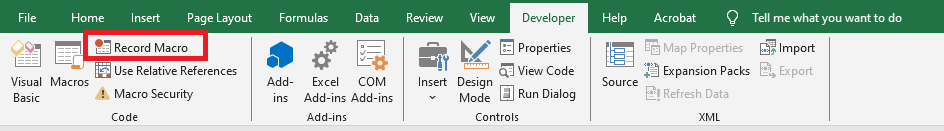
• To activate the macro recorder, go to the Developer tab on the ribbon, and in the Code group, click Record Macro.

In the Record Macro window that opens, set the required parameters for the recorded procedure: for example, assign the name ActivateSheet2 to the macro, enter appropriate explanations in the Description field, and leave the Store macro in field unchanged. Click OK.

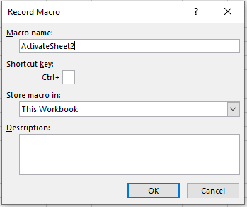
The Macro Name and Description fields are used to specify the macro’s name and its description. A macro name must not contain spaces, and the description is important for reusable macros, as over time it becomes difficult to remember why a given macro was created. By default, macros are named Macro1, Macro2, etc. To facilitate macro recognition, it’s better not to use a standard name but a unique one that describes its purpose.

In last Figure, notice the small box next to Ctrl+ in the Shortcut key section. You can place any letter of the alphabet in this field, and when pressed with the Ctrl key, it becomes a handy way to run the macro.

A shortcut key is not mandatory; in fact, most of your macros won’t need one. But if you choose to assign one, it’s best to use Ctrl+Shift+Key rather than just Ctrl+Key. Excel has already assigned Ctrl plus the 26 letters of the alphabet to built-in shortcuts for various tasks, and it’s best not to override them. For instance, Ctrl+C copies text. However, if you assign Ctrl+C to your macro, you will override the default function and lose the ability to use Ctrl+C to copy text in that workbook.
To use the shortcut key option, click the Shortcut Key field, press Shift, then a letter like S. You’ve now created the shortcut Ctrl+Shift+S, which won’t interfere with Excel’s main shortcuts.

The Store macro in dropdown allows you to select the workbook where the macro will be saved. If you select Personal Macro Workbook, the macro will be saved in a special hidden workbook where macros are stored. This workbook is always open but hidden, and the macros in it are available for other workbooks. To view your personal macro workbook, go to the View tab, and in the Window group, click Unhide.
If you select This Workbook (the default choice), the macro is stored in the active workbook. If you select New Workbook, it will be saved in a new workbook.

• While recording the macro, go to Sheet2 (the pointer is on cell A1).

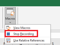
Click the Stop Recording button in the Code group under the Developer tab to stop recording the macro.6.

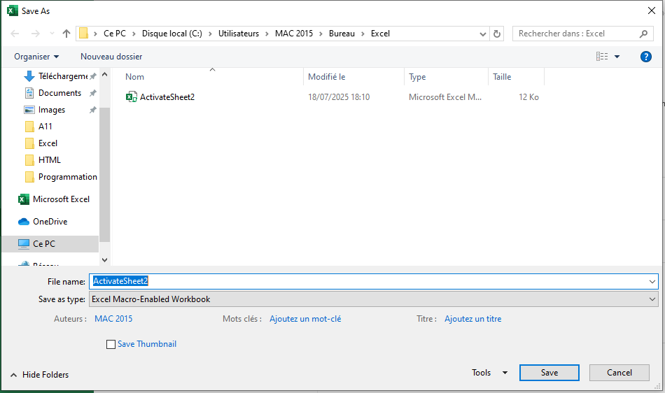
• Save your workbook in a format that supports macros: go to the File tab on the ribbon and select Save As. In the Save As dialog box (Figure 4), choose a save location, enter the workbook

name, and in the Save as type dropdown, choose Excel Macro-Enabled Workbook. Click Save.

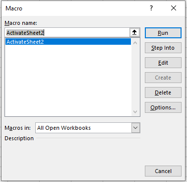
• Go to the Developer tab, click the Macros button in the Code group, and in the Macro window that opens, select your macro from the list (Figure 5) and click Edit.

The screen displays the VBA Editor with the standard module containing the macro code just recorded:

Sub ActivateSheet2() 
' 
' ActivateSheet2 Macro 
' 
   Sheets("Sheet2").Select 
End Sub

Notes

• A macro starts with the Sub statement and ends with End Sub. We’ll go deeper into macro structure in later chapters.
• ActivateSheet2() is the macro name.
• The instruction Sheets("Sheet2").Select is the macro body.

Now, without closing this workbook, create another workbook by going to the File tab, selecting New, and choosing Blank Workbook.

• Go to the Developer tab and click Macros in the Code group.
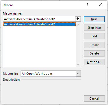
  In the Macro window (Figure 6), specify the name of the macro you created and click Run. Ensure that this macro activates Sheet2 in your workbook.

Assigning a Created Macro to a Button

Now let’s assign our created macro to a button placed on the Quick Access Toolbar. Follow these steps:

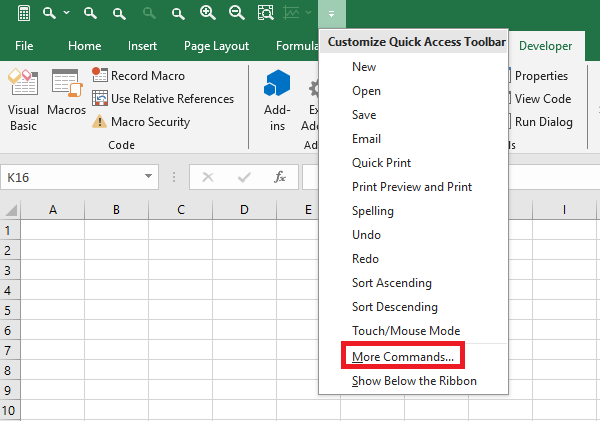
• Right-click on the Quick Access Toolbar and select More Commands… (Figure 7)

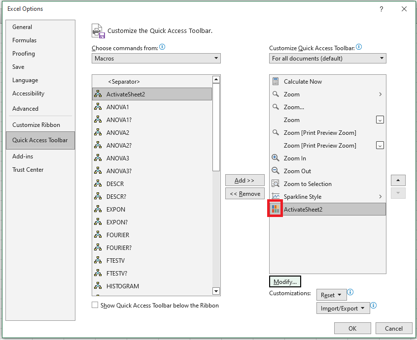
In the Excel Options window that opens, in the Quick Access Toolbar category, select Macros from the Choose commands from dropdown list .

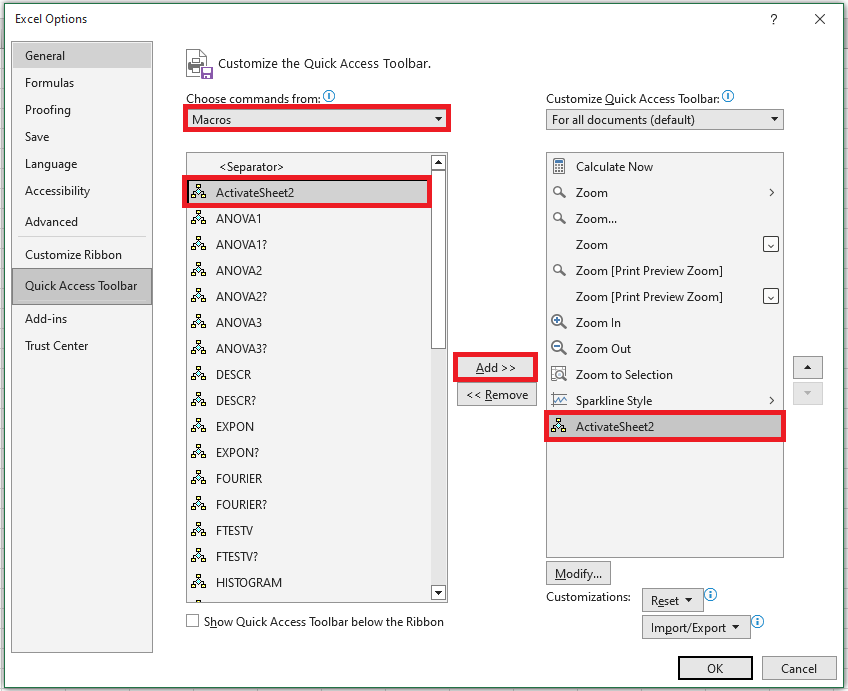
Select the macro ActivateSheet2 that you created in the left column and use the Add >> button to move it to the right column. Note that the Modify button is now available at the bottom of the right column—it’s used to assign an icon to the corresponding macro. Click the Modify button.

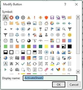
• In the Modify Button window that opens (Figure 9), choose a symbol for the button using your mouse and, if needed, in the Display Name field, edit the macro name. This display name will appear as a tooltip in the Quick Access Toolbar. Click OK.

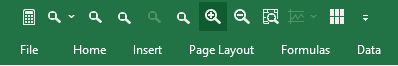
• In the Excel Options window under the Quick Access Toolbar category, the macro button appears in the right column (Figure 10). Click OK.
• Make sure the button with the recorded macro appears in the Quick Access Toolbar.

Automating Worksheet Tasks with Controls

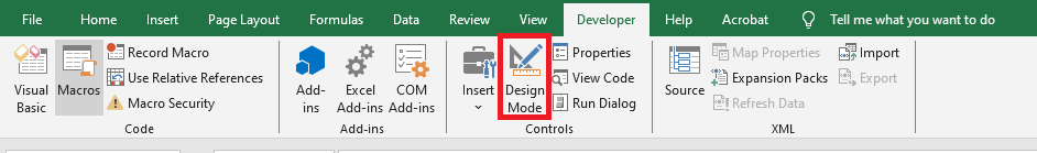
Excel also includes a complete set of controls—command buttons, text boxes, checkboxes, etc.—that you can place on a worksheet if needed. To view the available controls, go to the Developer tab, and in the Controls group, click the Insert button.

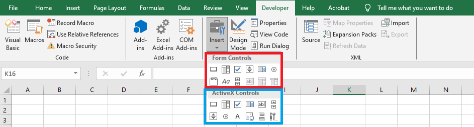
Note: the controls under the Form Controls group are primarily intended for compatibility with files from older Excel versions (up to Excel 97) that use these controls. They are much more limited in capability than the ActiveX Controls. Some of these form controls cannot be used at all in recent Excel documents (text box, list box, combo box). However, these controls have advantages not found in ActiveX controls—for example, they can be placed on chart sheets.

ActiveX controls are standalone components from various applications and can also be used in Microsoft Excel. This group includes controls similar to many in the Form Controls group (UserForm).

In addition to standard controls, you can use extra controls. Excel comes with several of these, such as multimedia controls that let you play sound or video directly from the worksheet. You can also connect controls from other programs or use custom-built controls.

In the worksheet module, you can create procedures that handle events triggered by these controls—for example, pressing a button, selecting a list item, checking an option box, etc. These actions can automatically trigger calculations, build charts, change chart types, and more.

Using a Command Button Control on a Worksheet

We’ll demonstrate how to use an ActiveX Command Button on a worksheet. Suppose that when we click the button, placed on Sheet1, Sheet2 is activated.

• Start Excel and make sure the cell pointer is on Sheet1.
• Go to the Developer tab, and in the Controls group, click the Insert dropdown list.
• Click on the Command Button (ActiveX Control) and move directly to the worksheet—your pointer turns into a thin cross.

Select a location on the worksheet, press the left mouse button, and while holding it, draw the button to the required size. Then release the button.
Note that once the Command Button appears on the sheet, Design Mode is activated.

On the first button’s surface, the default label CommandButton1 is automatically displayed (Figure 14). If you create a second Command Button now, it will be labeled CommandButton2, and so on.

NOTE:
Like any graphical object, a button can be drawn while holding Shift to give it a square shape, or Alt to snap it to the worksheet grid. With the sizing handles, you can adjust its dimensions, and with the move handle, you can set its position.

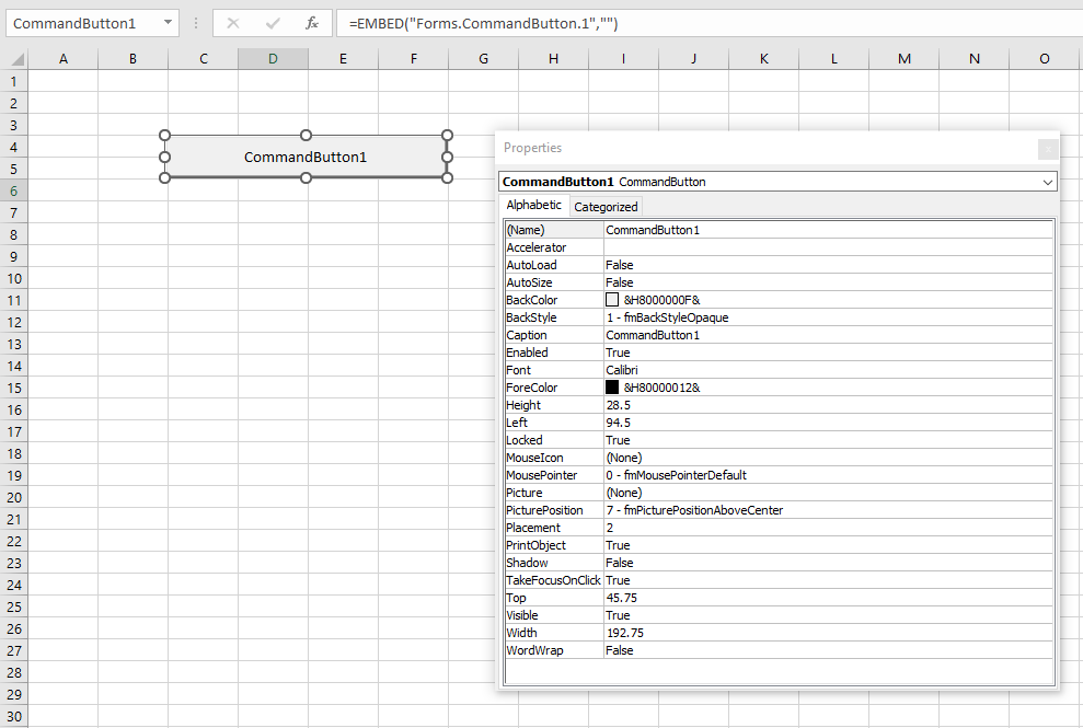
Right-click the created Command Button and in the context menu, select Properties to open the Properties window (see Figure 14). The Command Button is an object, meaning it has properties, methods, and events.

The Caption property sets the name displayed on the button surface. The Name property identifies the object in code. In this case, it’s also CommandButton1. In the Properties window, change the Caption from « CommandButton1 » to Sheet2 (to indicate that this button activates Sheet2). Optionally, test other properties: BackColor, Font, ForeColor, Shadow. Finally, close the Properties window.

• We’ll now write the procedure to handle the Click event. When the event is triggered, Sheet2 will be activated.
  Double-click the created Command Button (ensure Design Mode in the Developer tab is still active). This opens the VBA editor with the worksheet module for Sheet1, and automatically adds the starting and ending lines of the event procedure:

Private Sub CommandButton1_Click() 
End Sub

• Open the Windows file where you created the ActivateSheet2 macro. Make sure the required module is displayed in the VBAProject – Project Explorer window.
• Copy the macro’s line into the clipboard:

Sheets("Sheet2").Select

Of course, you could manually type it, but that’s slower and risks typos. Now insert that line inside the event procedure:

Private Sub 
   CommandButton1_Click() 
   Sheets("Sheet2").Select 
End Sub

Return to Sheet1. The button works only when Design Mode is off. So, click Design Mode in the Controls group on the Developer tab to deactivate it.
8. Test the created Command Button: click it. If everything was done correctly, it will activate Sheet2.

Another Example Using the Macro Recorder

Suppose you manage a data table daily, such as the one shown in the following figure, which displays the number of items sold by your company in its East, West, North, and South regions.

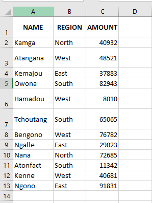
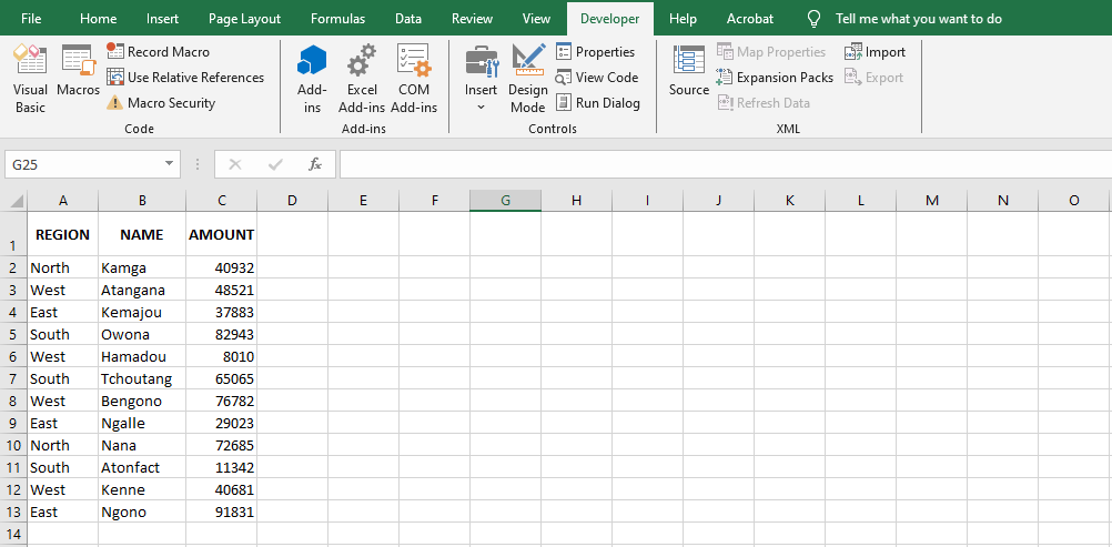
The daily task consists of sorting the table primarily by region, then by item. Your boss wants the columns NAME and REGION to switch places, so that REGION appears in column A and NAME in column B. To improve readability, the numbers in the AMOUNT column must be formatted with a comma separator, and the headers for REGION, NAME, and AMOUNT must be bolded. Next Figure16 shows the finished table, as requested by your boss.

This is normally a six-step process, which is quite tedious but part of your professional responsibilities.

NOTE

Whenever you create a macro, it’s a good idea to plan ahead: think about why you’re creating the macro and what you want the macro to do. This is especially important for complex macros, as you want your code to be efficient and accurate, using only the instructions necessary to get the job done properly. Avoiding excessive code will result in macros that run faster and are easier to edit or troubleshoot. For instance, prepare your workbook in advance to avoid recording unnecessary actions. Make sure the worksheet you’re working on is active and the relevant range is visible.

To complete the task, proceed as follows:

• Insert a new column at column A.
• Select the REGION column, cut it, and paste it into the new column A, to the left of NAME.
• Delete the now-empty column where REGION was.
• Select the range A1:C13 and sort in ascending order by REGION, NAME, and AMOUNT.
• Select range C2:C13 and format the AMOUNT values with a thousands separator.
• Select range A1:C1 and apply bold formatting to the headers.

These steps are not only repetitive but prone to human error. The good news is, if you perform the steps correctly while recording the macro, the task can be reduced to a single mouse click or keyboard shortcut, with VBA doing the heavy lifting for you.

To record the macro that performs this task, follow these steps:

• Start the macro recorder: go to the Developer tab on the ribbon and in the Code group, click Record Macro.
• In the Record Macro dialog box, enter "FormatData" in the Macro name field, select This Workbook for Store macro in, then click OK.
• Now perform the six steps listed above.
• Stop the macro recorder by clicking Stop Recording in the Code group on the Developer tab.

As a result, the following macro will be written to a standard module:

Sub FormatageDonnees()
' FormatageDonnees Macro
' Data Formatting

    Columns("A:A").Select
    Selection.Insert Shift:=xlToRight, CopyOrigin:=xlFormatFromLeftOrAbove

    Columns("C:C").Select
    Selection.Cut
    Columns("A:A").Select
    ActiveSheet.Paste

    Columns("C:C").Select
    Selection.Delete Shift:=xlToLeft

    Range("A1:C13").Select
    ActiveWorkbook.Worksheets("Sheet1").Sort.SortFields.Clear
    ActiveWorkbook.Worksheets("Sheet1").Sort.SortFields.Add Key:=Range("A2:A13"), _
        SortOn:=xlSortOnValues, Order:=xlAscending, DataOption:=xlSortNormal
    ActiveWorkbook.Worksheets("Sheet1").Sort.SortFields.Add Key:=Range("B2:B13"), _
        SortOn:=xlSortOnValues, Order:=xlAscending, DataOption:=xlSortNormal
    ActiveWorkbook.Worksheets("Sheet1").Sort.SortFields.Add Key:=Range("C2:C13"), _
        SortOn:=xlSortOnValues, Order:=xlAscending, DataOption:=xlSortNormal

    With ActiveWorkbook.Worksheets("Sheet1").Sort
        .SetRange Range("A1:C13")
        .Header = xlYes
        .MatchCase = False
        .Orientation = xlTopToBottom
        .SortMethod = xlPinYin
        .Apply
    End With

    Range("C2:C13").Select
    Selection.NumberFormat = "#,##0"

    Range("A1:C1").Select
    Selection.Font.Bold = True
End Sub

Comments

• As seen before, all macros begin with a Sub statement (short for Subroutine, commonly known as a macro), which includes the macro name followed by parentheses.
• The comments you see in a recorded macro reflect the information entered in the Record Macro dialog box. For example, if you assign a shortcut key or enter a description, these appear as comments in the code.
• The remaining lines are VBA instructions representing every action performed while recording the macro.

Here’s a breakdown:

• You selected column A.
• You inserted a new column.
• You selected column C, cut it, and pasted it into column A.
• You selected the now-empty column C and deleted it.
• You selected range A1:C13 (the data table).
• You sorted the data.
• You selected C2:C13 to format the numbers.
• You applied a thousands separator.
• You selected A1:C1 for the headers.
• You bolded the font in those cells.
• You stopped the macro recording, which ends with End Sub.

Improving the Recorded Macro

It’s easy to generate a macro with the Record Macro button. However, the recorded macro often lacks efficiency and produces unnecessary code. To be fair, the Record Macro tool isn’t designed to write optimized code. Its purpose is to produce VBA code that mirrors your on-screen actions exactly.

There’s no rule that says you must always clean up your recorded macros. For simple tasks that work as intended, keeping them as-is can be perfectly fine.

However, for most recorded VBA code, the unnecessary and inefficient parts can’t be ignored. Moreover, if you plan to share your VBA work, you’ll want it to look clean and professional.

A key VBA development principle is: Avoid Select and Activate unless necessary. These are often the main reason for slow-running macros.

For example, these two recorded lines:

Columns("A:A").Select
Selection.Insert Shift:=xlToRight

Can and should be simplified to:

Columns("A").Insert Shift:=xlToRight

Similarly, this code:

Columns("C:C").Select
Selection.Cut
Columns("A:A").Select
ActiveSheet.Paste

Can be replaced with:

Columns("C").Cut Destination:=Columns("A")

And this code:

Columns("C:C").Select
Selection.Delete Shift:=xlToLeft

Can be simplified to:

Columns("C").Delete Shift:=xlToLeft

By streamlining the code, your FormatData macro becomes more readable and much more efficient.