The F-test is a statistical hypothesis testing procedure used to compare the variances of two independent samples. It is primarily applied when we need to assess whether the variability (or spread) of two datasets is significantly different. This test helps determine whether the two samples can be assumed to come from normal populations that share the same variance.
In practical applications, the F-test is valuable in many fields. For instance, a quality control analyst may use it to evaluate whether product quality is deteriorating over time by comparing the variances of product measurements taken at different time intervals. Similarly, an economist might apply the F-test to compare the variability of income levels between two demographic groups or regions.
Excel offers built-in tools and functions (such as F.TEST, F.DIST, and F.INV) that make performing the F-test accessible and straightforward for users who wish to conduct variance comparisons within their datasets.
Key Takeaways
-
■ The F-test is a statistical method used to evaluate whether the variances of two normally distributed populations are equal.
-
■ It is based on the F-ratio, which is the ratio of the two sample variances.
-
■ If the computed F-value is relatively small (e.g., F < 0.5), it may suggest that there is no significant difference between the variances, indicating the samples could belong to populations with similar variability.
-
■ Conversely, if F ≥ F₀.₅ (a critical value from the F-distribution table at the 0.5 level), the null hypothesis — which assumes equal variances — is rejected, meaning the difference in variances is statistically significant.
-
■ F-test vs. t-test: While both are statistical tests, they serve different purposes. The t-test compares the means of two samples, whereas the F-test compares their variances. Both are essential tools in statistical inference but answer different research questions.
Explanation of the F-Test in Statistics
The F-test is a fundamental statistical method used to determine whether the variances of two populations are equal. It is often referred to as the variance ratio test because it involves calculating the ratio of two sample variances. The main objective is to evaluate whether the observed difference in variability between two groups is statistically significant.
The F-test was first introduced by the British statistician Ronald A. Fisher, after whom the test is named. It was later formalized and expanded upon by George W. Snedecor, who helped develop its practical applications in statistical analysis.
Conditions Required for the Valid Use of the F-Test
To ensure the validity of the F-test when comparing the variances of two populations, the following assumptions and conditions must be satisfied:
-
■ Normality:
Both populations being compared must follow a normal distribution. If the data are not normally distributed, the results of the F-test may be unreliable or invalid. -
■ Independent and Random Sampling:
The elements selected for each sample must be independent of each other and chosen through a random process. This helps avoid bias and ensures the representativeness of the sample. -
■ Variance Ratio ≥ 1:
The F-test is designed so that the larger sample variance is divided by the smaller one, ensuring that the variance ratio (F) is greater than or equal to 1. This convention simplifies interpretation and aligns with the F-distribution, which is skewed and only defined for positive values. -
■ Additive Property of Variance:
The total variance observed in the data is assumed to be the sum of two components:-
The variance between the samples (i.e., differences due to group membership)
-
The variance within the samples (i.e., random variation within each group)
This principle is especially important in Analysis of Variance (ANOVA), where the F-test plays a central role in decomposing and analyzing sources of variation.
-
The F-Test Formula and Its Application
Sample Variance Formula
In the context of the F-test, we begin by calculating the sample variances of the two groups. The formula for sample variance (denoted as S2S^2) is:
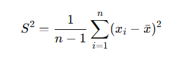
Where:
-
n is the sample size
-
xi is each individual value
-
xˉ is the sample mean
To simplify this process, you may use an online F-test calculator, which performs all the computations automatically.
Null Hypothesis ( H0 )
When performing an F-test, the null hypothesis is formulated as follows:
-
H0: The two populations have equal variances, i.e.,
σ12=σ22
This can be interpreted in two ways:
-
(a) The two samples come from the same population
-
(b) The population variances are equal, even if the samples differ
Variance Ratio Formula
To compute the F-statistic, we use the formula:
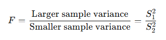
Note: Whether S12 or S22 is in the numerator depends solely on which is larger. This ensures the F-value is always ≥ 1.
Degrees of Freedom (df)
-
For the numerator (larger variance): df1=n1−1
-
For the denominator (smaller variance): df2=n2−1
These values are used to find the critical value from the F-distribution table, based on a chosen significance level (e.g., 5%).
Decision Criteria
Compare the calculated F-value with the critical F-value from the F-table:
-
If F≤F0.05, the result is not statistically significant. We fail to reject the null hypothesis and conclude that the variances are likely equal.
-
If F>F0.05, the result is statistically significant. We reject the null hypothesis and conclude that the variances are different.
Example: Comparing Incomes in Two Villages
| Village | A | B |
|---|---|---|
| Sample Size (nn) | 10 | 12 |
| Mean Monthly Income | 150 | 140 |
| Sample Standard Deviation | 92 | 110 |
Step 1: Calculate Sample Variances
We square the sample standard deviations:
S12=922=8464 and S22=1102=12100
Now, place the larger variance in the numerator:
F=12100/8464≈1.43
Step 2: Determine Degrees of Freedom
-
df1=12−1=11
-
df2=10−1=9
Step 3: Look Up the Critical Value
Using the F-distribution table at a 5% significance level, the critical value for df1=11 and is approximately 2.90.
Step 4: Interpret the Results
Fcalculated=1.43 < Fcritical=2.90
Since the calculated F-value is less than the critical value, we fail to reject the null hypothesis.
How to Perform an F-Test in Excel
The F-Test is used to compare the variances of two data sets and determine whether they are significantly different. This type of test is useful when assessing the assumption of equal variances in statistical analyses such as ANOVA or t-tests.
Here are the step-by-step instructions to perform an F-Test in Microsoft Excel using the Data Analysis Toolpak:
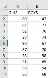
Step 1: Prepare your data
Make sure your data is organized in two separate columns, each representing one of the two data sets (variables) you want to compare. For example:
-
Column A: Variable 1 (e.g., Sample A)
-
Column B: Variable 2 (e.g., Sample B)
Ensure that each column contains numerical values and that both variables have the same number of observations.
Step 2: Enable the Data Analysis Toolpak
Before performing the F-Test, make sure the Data Analysis Toolpak is installed and activated:
-
Go to the « File » menu, then select « Options »
-
Click on « Add-ins »
-
In the « Manage » box at the bottom, choose « Excel Add-ins » and click « Go »
-
Check « Analysis ToolPak » and click « OK »
Once activated, a new option called « Data Analysis » will appear in the « Data » tab on the ribbon.

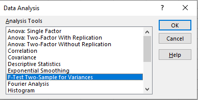
Step 3: Launch the F-Test procedure
-
Go to the « Data » tab in the Excel ribbon.
-
Click on « Data Analysis » (usually located on the right side of the ribbon).
-
In the dialog box that appears, scroll down and select « F-Test Two-Sample for Variances », then click « OK ».
Step 4: Input your data ranges
In the F-Test dialog box:
-
For Variable 1 Range, select the range of cells that contains the first set of data (e.g.,
A2:A11) -
For Variable 2 Range, select the range of the second data set (e.g.,
B2:B11) -
If your data includes headers (e.g., « Sample A », « Sample B »), check the « Labels » box
-
Choose a significance level (commonly 0.05 for a 5% significance level)
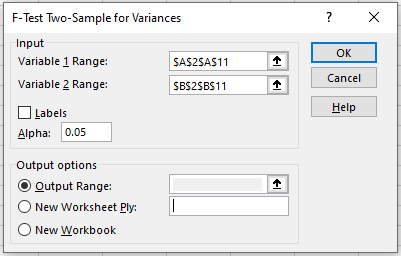
Step 5: Choose an output option
-
Select an Output Range if you want the results to appear within the worksheet, or
-
Choose New Worksheet Ply to display the results on a separate sheet
Step 6: Click « OK » to run the test
Once you click « OK », Excel will display the F-Test results in the designated output area. The key results to interpret include:
-
F (test statistic): the ratio of the two variances
-
P(F ≤ f) one-tail: the p-value used to determine significance
-
F Critical one-tail: the critical value at your chosen alpha level
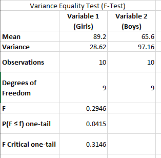
Interpreting the results
Compare the calculated F value to the F critical value:
-
If F > F Critical, the variances are significantly different
-
Alternatively, if the p-value is less than the significance level (e.g., 0.05), you reject the null hypothesis of equal variances
Understanding the F-Test: Purpose, Functioning, and Applications
What is the F-Test and When Is It Used?
The F-test is a statistical procedure used to compare the variances of two datasets to determine if they are significantly different from one another. It helps answer the question: Are the variances of two populations equal or not? This test is commonly employed in the context of variance analysis and is essential for conducting ANOVA (Analysis of Variance).
How the F-Test Works
The key elements of the F-test are outlined below:
-
The F-test is applied when we want to test for a significant difference between the variances of two data samples.
-
The null hypothesis (H₀) assumes that the variances of the two datasets are equal.
-
The alternative hypothesis (H₁) assumes that the variances are different.
-
If the calculated F-value is significantly large and the p-value is below the chosen level of significance (usually 0.05), we reject the null hypothesis, indicating that the variances differ.
-
If the p-value is above the threshold, we fail to reject the null hypothesis, suggesting the variances are statistically equal.
Limitations and Requirements of the F-Test
-
The F-test requires two datasets; it cannot be conducted on a single sample.
-
It returns an error in the following cases:
-
If either dataset contains fewer than two values.
-
If the variance of one of the datasets is zero, making comparison meaningless.
-
-
The F-test ignores non-numeric data such as text values and focuses solely on the numerical variances.
Typical Applications of the F-Test
The F-test is commonly used in scenarios where comparing variability is crucial. Examples include:
-
Evaluating the teaching effectiveness of two professors delivering the same course by comparing the variance in students’ performance.
-
Comparing two samples of bottled water (or gourds) tested under different environmental conditions.
-
Analyzing test scores from two groups of students within the same academic field to assess consistency.
F-Test vs T-Test: Key Differences
| Feature | T-Test | F-Test |
|---|---|---|
| Purpose | Tests for significant difference between means of two datasets. | Tests for significant difference between variances of two datasets. |
| Null Hypothesis (H₀) | The means of the two populations are equal. | The variances of the two populations are equal. |
| Focus | Determines whether a single variable is statistically significant. | Determines whether a group of variables is collectively significant. |
| Degrees of Freedom (df) | df=n−1, where n is the sample size. | df1=n1−1, df2=n2−1, where n₁ and n₂ are sample sizes of the two datasets. |
Is the F-Test the Same as ANOVA?
The F-test is a general term for any statistical test that uses an F-statistic to compare variances. ANOVA (Analysis of Variance) is a specific application of the F-test used to compare the means of three or more groups. ANOVA relies on the assumption that the populations are normally distributed, have equal variances, and are independent.
In summary:
-
Every ANOVA involves an F-test.
-
Not every F-test is an ANOVA.
Understanding the P-Value in the F-Test
The P-value in an F-test represents the probability that the observed differences in variance could have occurred by random chance.
-
A small p-value (typically < 0.05) indicates strong evidence against the null hypothesis, suggesting that the variances are significantly different.
-
A large p-value (typically > 0.05) implies weak evidence against the null hypothesis, supporting the idea that the variances are equal.
For example:
-
A p-value of 0.01 means there is a 1% chance that the variance difference occurred randomly.
P-values are also used to determine the statistical significance of individual variables within a dataset.