Here’s a very simple and concise definition of a circular reference provided by Microsoft:
« When an Excel formula refers to its own cell, either directly or indirectly, it creates a circular reference. »
For example, if you select cell A1 and type =A1, that creates a circular reference in Excel.
Typing any other formula that refers to A1, such as =A1*5 or =IF(A1=1, "OK", ""), would have the same effect.
As soon as you press Enter to complete such a formula, you’ll see the following warning message:
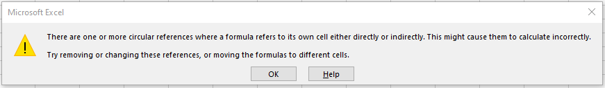
Why Does Excel Warn You?
Because circular references can cause infinite loops, slowing down your workbook’s calculations significantly.
After you receive the warning, you can click Help for more info or close the message window by clicking OK or the X button.
Once the window is closed, Excel displays either zero (0) or the last successfully calculated value in the cell.
In some cases, a formula with a circular reference may complete successfully before it begins recalculating, and when that happens, Excel returns the last known valid value.
When you enter multiple formulas with circular references, Excel doesn’t always show the warning repeatedly.
But Why Would Anyone Create Such a Problematic Formula?
Sometimes, you may accidentally create a circular reference. Here’s a very common scenario:
Suppose you want to sum the values in column A using the SUM function, and you inadvertently include the total cell itself (e.g., B6) in the sum range.
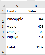
If circular references are not allowed in your Excel (they’re disabled by default), you’ll see an error message.
If iterative calculations are enabled, your circular formula will return 0, as shown above.
Sometimes, blue arrows may also suddenly appear in your worksheet, making it look like Excel is acting up.
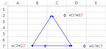
Actually, these arrows are just Trace Precedents or Trace Dependents tools that indicate which cells influence or are influenced by the active cell.
Are Circular References Always Bad?
At this point, you may feel like circular references are completely useless and dangerous, and wonder why Excel allows them at all.
However, there are rare cases where a circular reference can provide a shorter and more elegant solution.
Example: Using a Circular Reference in Excel
Suppose you have a list of items in column A, and you enter a delivery status in column B.
As soon as you type “Yes” in column B, you want the current date and time to be automatically entered in column C on the same row — as a static, unchanging timestamp.
Using the NOW() function isn’t an option because it’s volatile and updates every time the sheet is recalculated.
A better solution is to use nested IF functions with a circular reference like this:=IF(B3="YES", IF(C3="", NOW(), C3), "")
Where B3 is the delivery status and C3 is where the timestamp appears.
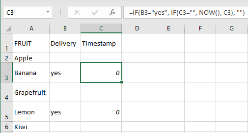
In this formula, the first IF checks cell B3 for “YES” and, if true, runs the second IF.
If false, it returns an empty string.
The second IF is a circular formula that captures the current date and time only if C3 is empty — preserving all existing timestamps.
Note:
For this formula to work, you must enable iterative calculations in your worksheet — which we’ll cover next.
How to Enable/Disable Circular References
As mentioned, iterative calculations are turned off by default in Excel.
(Iteration means repeated recalculation until a specific numeric condition is met.)
To enable circular formulas to function, you need to activate iterative calculation in your workbook.
In Excel 2019, 2016, 2013, or 2010:
- Go to File > Options
- Select Formulas
- Check the box Enable iterative calculation under Calculation options
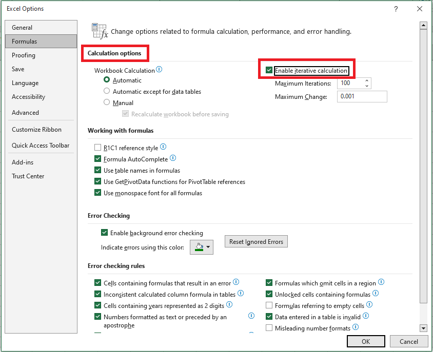
When you enable iterative calculation, you must define two settings:
■ Maximum Iterations – The number of times a formula should recalculate. Higher numbers slow down performance.
■ Maximum Change – The minimum amount of change between calculation results. Smaller numbers improve accuracy but increase time.
The default settings are:
- Maximum Iterations: 100
- Maximum Change: 0.001
This means Excel will stop recalculating your circular formula after 100 iterations or when the result changes by less than 0.001, whichever comes first.
Why You Should Avoid Circular References
As you’ve seen, circular references are generally a risky and discouraged practice in Excel.
In addition to:
- Slower performance
- Warning messages every time the workbook opens (unless iteration is enabled)
They may also create invisible problems.
For example, if you:
- Select a cell with a circular reference
- Accidentally press F2 (Edit mode)
- And press Enter without making changes
→ The formula will recalculate and return0.
Tip from Excel experts:
Avoid circular references as much as possible in your worksheets.
How to Find Circular References in Excel
To locate circular references in your workbook:
- Go to the Formulas tab
- Click the arrow next to Error Checking, then hover over Circular References
- The last circular reference entered will be listed
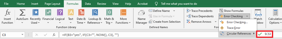
- Click the listed cell and Excel will take you directly to it.
The status bar will show a message indicating circular references were found and display the address of one such cell.
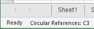
Note:
If circular references exist in another sheet, the status bar will only display “Circular References” without a cell address.
This feature is disabled when iterative calculation is turned on, so you must disable it first to locate circular references.
How to Remove Circular References
Unfortunately, Excel does not offer a one-click solution to remove all circular references in a workbook.
You need to:
- Inspect each circular reference manually (as shown above)
- Either delete the formula
- Or replace it with one or more simpler, non-circular formulas
How to Trace Relationships Between Formulas and Cells
When a circular reference isn’t obvious, the Trace Precedents and Trace Dependents tools can help.
They draw lines showing which cells affect or are affected by the selected cell.
To view these arrows:
- Go to the Formulas tab
- In the Formula Auditing group, click:
- Trace Precedents – Shows which cells provide data to the formula (i.e., which cells influence the selected cell)
- Trace Dependents – Shows which cells depend on the selected cell (i.e., which formulas refer to it)
To hide the arrows, click Remove Arrows (located under Trace Dependents).
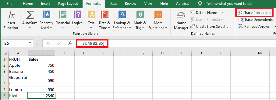
In the example above, the Trace Precedents arrow shows which cells feed into B6.
As you can see, B6 is included in its own formula, creating a circular reference that returns zero.
This case is easy to fix—simply replace B6 with B5 in the SUM argument:=SUM(B2:B5)
Other circular references might not be so obvious and require more thought and calculation.