Excel tables are among the most powerful features for managing, calculating, and updating structured datasets efficiently. While tables provide enhanced functionality like automatic expansion, structured references, and built-in filters, there may be cases where you need to revert a table back to a regular range—or convert a standard range into a fully functional table.
How to Convert an Excel Table to a Normal Range
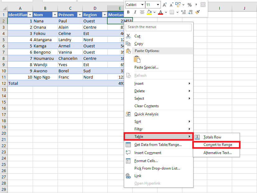
If you wish to remove table functionality while keeping your data intact, Excel offers a quick way to convert a table into a normal range. Follow these steps:
- Method 1 (Right-click method):
Right-click any cell within the table. From the context menu, select Table > Convert to Range.
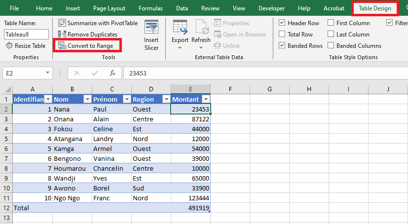
- Method 2 (Using the Ribbon):
- Select any cell in the table to activate the Table Design tab.
- On the Table Design tab (formerly « Design » in older versions), locate the Tools group and click Convert to Range.
In both cases, Excel will prompt you with a confirmation dialog.
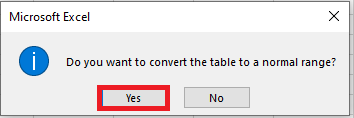
Click Yes to proceed. Once confirmed, the table will be converted to a regular range.
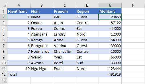
Note that while this process removes table-specific features—such as automatic column expansion, structured formulas, and filter buttons—it preserves the visual formatting (e.g., font colors, cell fill, and borders) applied by the table style.
Converting a Normal Range to an Excel Table
To leverage the full capabilities of Excel tables, you can convert any range of data into a table. There are multiple ways to do this:
- Quick Shortcut Method:
- Select any cell within your data range.
- Press Ctrl + L (or Ctrl + T in newer versions).
-
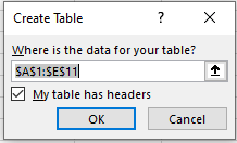
- In the Create Table dialog box, verify the selected range. If your data includes headers, ensure the My table has headers checkbox is selected.
- Click OK.
The selected range will instantly become an Excel table, adopting the default table style.
Using the Ribbon to Create a Table
You can also create a table using the ribbon interface:
- Select any cell within your dataset.
- Go to the Insert tab.
- In the Tables group, click Table.
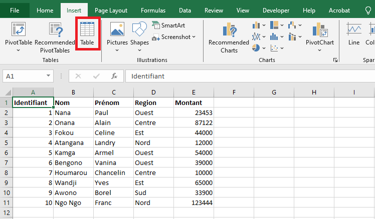
- In the Create Table dialog box, confirm the range and header option, then click OK.
Just like the shortcut method, this action transforms your range into a table with the default style applied.
Converting a Range to a Table with a Specific Style
If you want to apply a specific visual style to your new table right from the beginning, proceed as follows:
- Select any cell within your dataset.
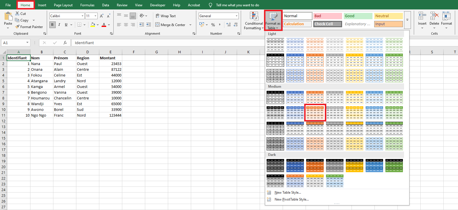
- Navigate to the Home tab.
- In the Styles group, click Format as Table.
- Choose your preferred table style from the gallery.
- In the Create Table dialog, confirm the selected range and whether it contains headers, then click OK.
The selected range is now formatted as a table using the chosen style.
If your dataset already has custom formatting and you want to apply the table style without conflicts, you can right-click the style in the gallery and select Apply and Clear Formatting. This option will remove any existing formatting before applying the table style, ensuring consistency and avoiding design clashes.