How to create dynamic chart labels?
You’ve probably encountered workbooks containing charts where you edit a worksheet entry, and the chart labels don’t change. This often creates confusion. Now learn how to link series labels and chart titles to worksheet cells. Suppose you want to plot future GDP in the United States (US) and China. You want the chart title to contain the year in which Chinese GDP exceeds US GDP, and the series label to contain each country’s annual growth rate . In C5 and C8, you can change the estimated growth rates from their current values of 3% for US GDP and 10% for Chinese GDP.
Create dynamic labels.
The goal is to link your chart title and labels to cells that change when growth rates change. Do the following:
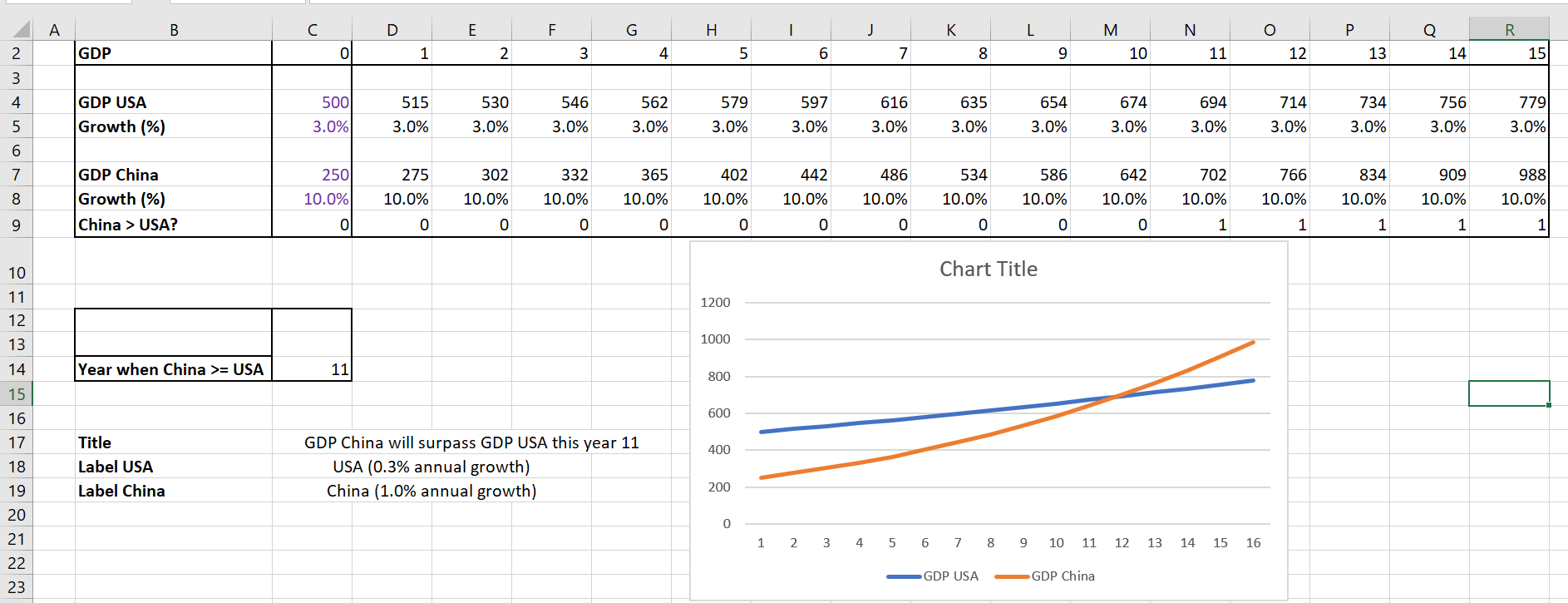
1. Copy the formula IF (D7>=D4;1;0) from D10 to E10: R10 enters a 1 if the Chinese GDP is greater than the US GDP.
2. In cell C14, determine the year in which China overtakes the United States with the formula =IFERROR(MATCH( 1,D 10:R10,0); »none »). Note that if China never overtakes the United States, this formula returns none .
3. In cell C17, the formula = IF( S15= »none »; « US Remains Leading »; « China’s GDP will overtake US GDP this year » &TEXT(C14, »0″)) creates the desired chart title. Note that if China never overtakes the US, your chart title will be US Remains Leading . Otherwise, your chart title is tied to C14, so the chart title will contain the year in which China overtakes the US. The » 0″ in the TEXT function ensures that the year is formatted as an integer.
4. In cell C18, the formula = « USA(« &TEXT(C5, »0.0% »)& » annual growth) » creates the chart title for the USA series. The « 0.0 % » part of the text function ensures that the growth rate is formatted as a percentage.
5. In cell C19, the formula = « China(« &TEXT(C 8, « 0.0% »)& » annual growth) » creates the chart title for the China series.
6. You are now ready to create the chart with dynamic labels.
7. Press Ctrl, select the non-continuous range C2 : R2 , C4:R4 , C7:R7 and create a scatter plot (third option).
8. Select Add Chart Element on the Design tab and select Chart Title / Centered Overlay . In the formula bar, type an equal sign (=), point to cell C17 and press Enter . You now have a dynamic chart label.
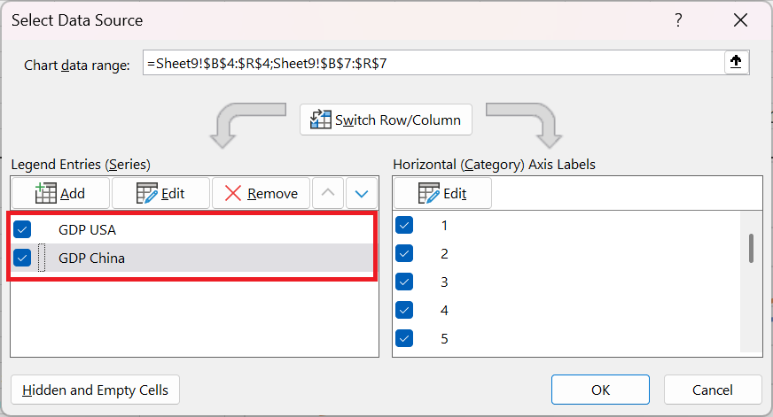
9. Select the USA data series and right-click and choose Select Data . Click Edit & Fill in the Edit Series dialog box as follows:
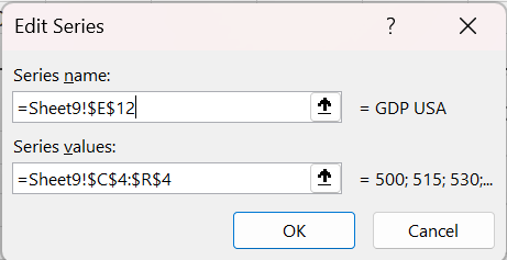
Create a dynamic label for the USA series.
This links the USA series label to cell C18, which contains the annual growth rate. Similarly, you link the China series label to cell C19, as shown in the following figure.
You have now completed a chart with dynamic labels.