Displaying Multiple Views Through a Chart
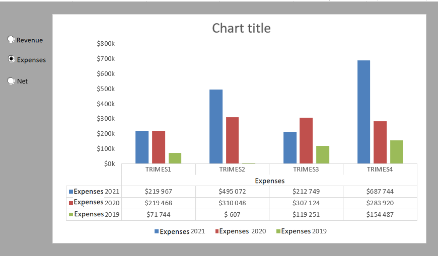
One way to use radio buttons is to populate a single chart with different data , depending on the option selected. The following figure illustrates an example. As each category is selected, the single chart is updated to display the data for that selection.
This chart is dynamically populated with different data depending on the radio button selected.
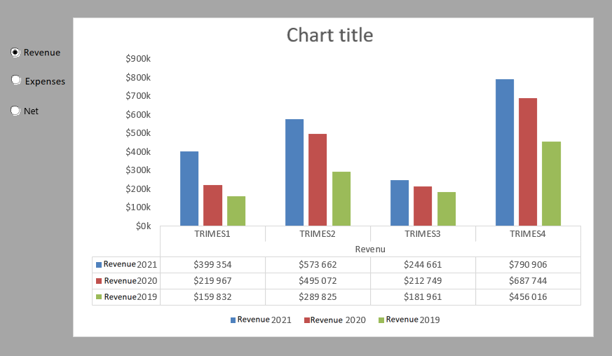
Now, you can create three separate charts and display them all on your dashboard at the same time. However, using radio buttons as an alternative saves valuable real estate by not having to display three separate charts. In addition, it is much easier to troubleshoot , format, and maintain one chart than three.
To create this example, start with three raw datasets—as shown in the following figure—containing three categories of data ; Income, Expenses, and Net. The radio button controls display their values in cell A8. This cell contains the ID of the selected option: 1, 2, or 3.
Raw datasets and a cell where radio buttons can display their values.
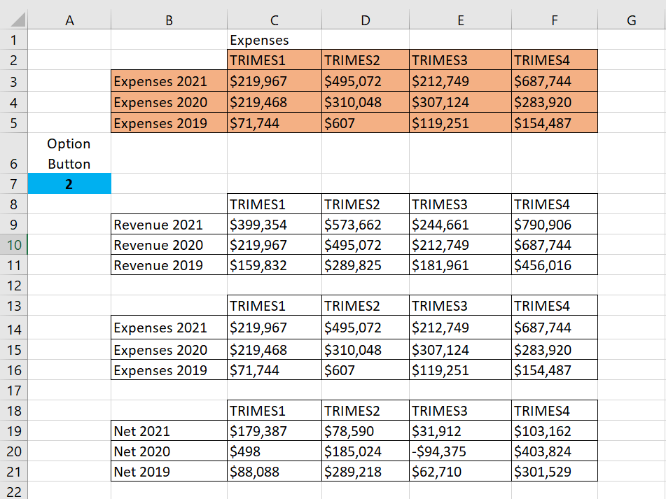
You then create the analysis layer (the staging table) consisting of all the formulas, as shown in the following figure. The chart is bound to the data in the staging table, which allows you to control what the chart sees. The first cell in the staging table contains the following formula:
=IF ($A$8 = 1; B9; IF ($A$8 = 2; B13; B17))
Create a staging table and enter this formula in
the first cell.
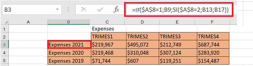
This formula tells Excel to check the value in cell A8 (the cell where the option buttons display their values). If the value in cell A8 is 1, which represents the value of the Income option, the formula returns the value in the Income dataset (cell B9). If the value in cell A8 is 2, which represents the value of the Expenses option , the formula returns the value in the Expenses dataset (cell B13). If the value in cell A8 is not 1 or 2, the value in cell B17 is returned.
Note that the formula shown in the following figure uses absolute references with cell A8. That is, the reference to cell A8 in the formula is prefixed with dollar signs ($A$8). This ensures that cell references in formulas do not change when copied and traversed.
To verify that the formula is working correctly, you can manually change the value in cell A8, from 1 to 3. When the formula works, you simply copy the formula to fill the rest of the staging table. Once the configuration is created, all that’s left is to create the chart using the staging table.