Track sales performance over time
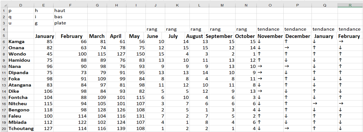
You want to use icons (up, down, or flat arrow) to track during each month whether a seller’s ranking improved, decreased, or remained the same.
You can use Excel icon sets, but then you’ll have to insert a set of icons for each month, which is a tedious task. A more efficient way to create these icons is to enter an h when you want an up arrow, enter an i when you want a down arrow, and enter a g when you want a flat arrow. Then, if you change the font to Wingdings 3, you have the desired arrows because the letters of the alphabet in Wingdings 3 correspond to the symbols shown in the following figure.
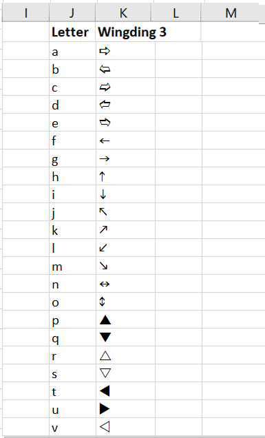
This is the correspondence between the letters and the Wingdings 3 symbols.
To create the icons shown in Figure 20 , follow these steps:
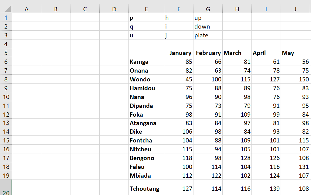
■ Copying the formula RANK( E6; E$6:E0; 0) from J6 to J6:N20 calculates the sales rank of each person during each month.
■ Copy of the SI formula (K6 <J6; « h » ; IF (K6> J6 ; « i » ; « g « )) from O6 to O7 : R20 creates an h if the person’s rank has improved, an i if the person’s rank has decreased, and ag if the seller’s rank has remained the same.
■ After changing the font of the range O 6: R20 to Wingdings 3, you see the icons displayed in the following.
The advantage of this approach is that you can use if statements to customize the conditions that define the icons.