Use an image to replace data bars
Typically, product sales are summarized using boring columns or bars, where the column height or bar width is proportional to the product sales. Wouldn’t it be more fun to summarize product sales with a picture of your product, proportional to actual sales? To illustrate the idea, check out the Using a Picture spreadsheet and the chart shown in the following figure.
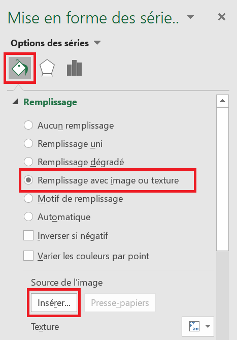
In this example, you assume that your company sells Coca-Cola, so you want to summarize the monthly sales with a Coca-Cola bottle whose size reflects the magnitude of the monthly sales. To begin, select the C 5: D12 and in the Insert tab, select the first 2D column chart option (Clustered Column). Then right-click on a column and Format Data Series . In the dialog box that appears, go to the Fill option and select Fill with a picture or texture , as shown in the following figure.
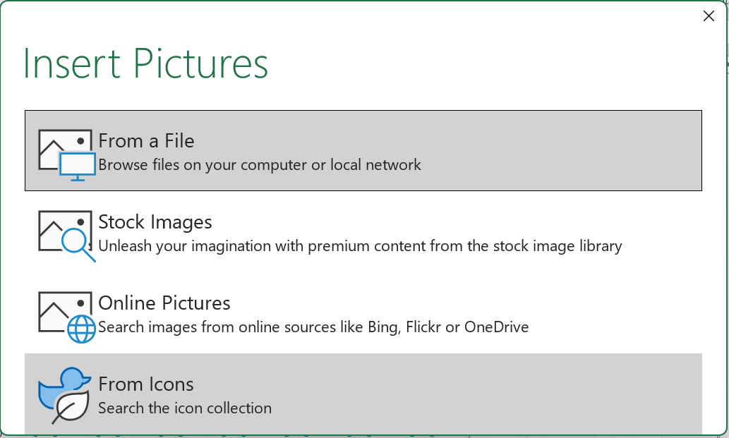
Below the Image Source heading , click Insert , and you will see the window shown in the following figure. After selecting the desired Coca-Cola bottle and clicking Insert, the image is inserted into the chart, with the height of the Coca-Cola bottle being proportional to the actual sales.
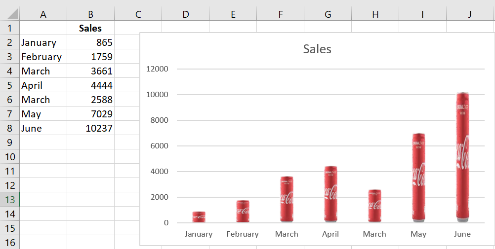
Coca-Cola sales are summarized with a bottle of Coca-Cola.