How to Use Conditional Formatting in Excel

How to Use Conditional Formatting in Excel

Conditional formatting in Excel is a very powerful feature when it comes to applying different formats to data that meets certain conditions. It can help you highlight the most important information in your spreadsheets and identify discrepancies in cell values at a glance.

At the same time, conditional formatting is often considered one of the most complex and obscure Excel functions, especially by beginners. If you also feel intimidated by this feature, don’t! In fact, conditional formatting in Excel is very simple and easy to use, and you’ll be sure to master it in just 5 minutes once you finish reading this short tutorial.

1 The Basics of Conditional Formatting

Similar to regular cell formats, you use conditional formatting in Excel to format your data in different ways by changing the fill color, font color, and border styles of cells. The difference is that conditional formatting is more flexible, allowing you to format only data that meets certain criteria or conditions.

You can apply conditional formatting to one or more cells, rows, columns, or the entire table based on the cell’s contents or the value of another cell. To do this, create rules (conditions) in which you define when and how selected cells should be formatted.

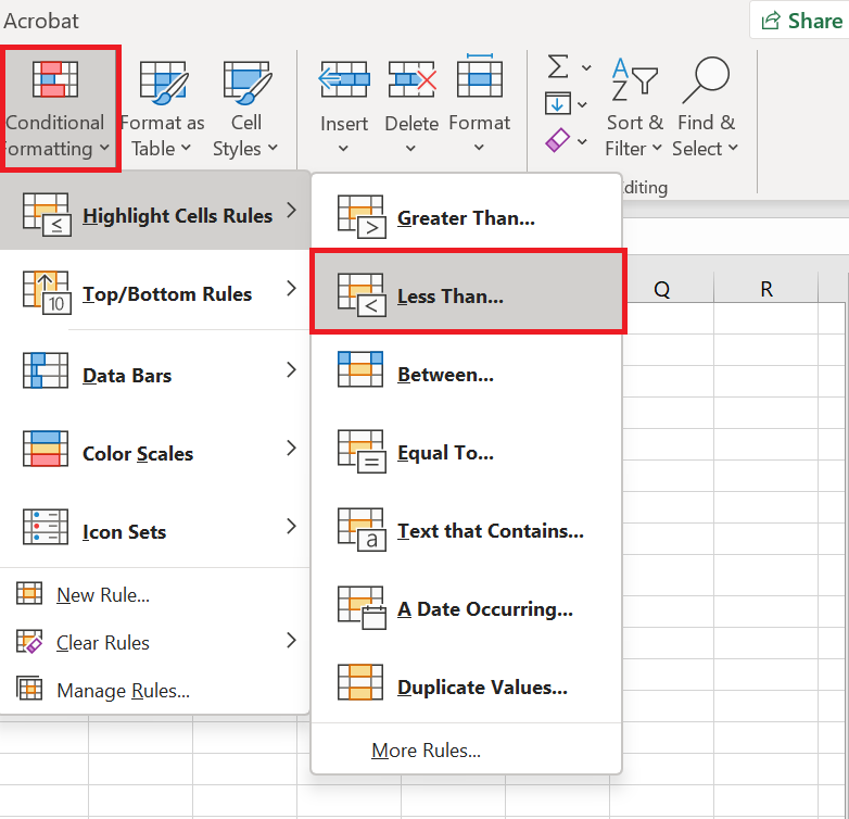
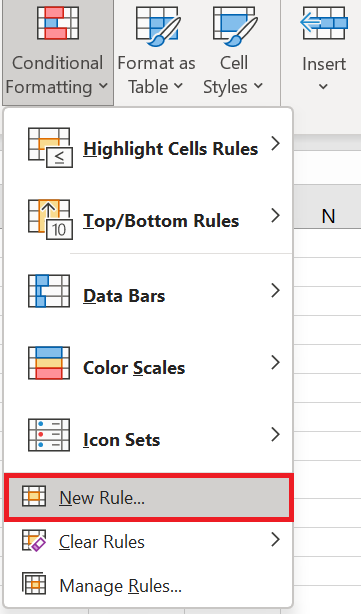
To begin, let’s see where you can find the conditional formatting feature in different versions of Excel. And the good news is that in all modern versions of Excel, conditional formatting resides in the same location, in the Home tab / Styles group , click Conditional Formatting .

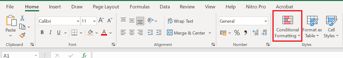
This figure shows the conditional formatting command.

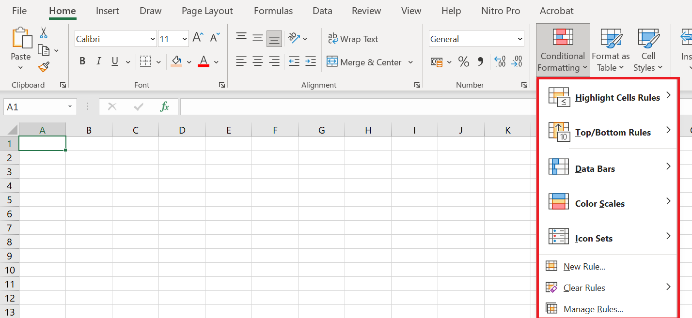
Here is a brief explanation of each option:

■ Cell Highlighting Rules: These rules allow you to assign a format to cells whose content meets one of the following criteria:

• Are in a specific numeric range

• Match a specific text string

• Are within a specific date range (relative to the current date)

• Occur multiple times (or only once) in the selected range

■ High/Low Range Value Rules : Use these rules to assign a format to any of the following:

• N largest or smallest values in a range. For example, N = 10 will highlight the 10 largest or 10 smallest values in a range.

• Upper or lower percentage of numbers in a range.

• Numbers greater than or less than the average of all numbers in a range.

■ Data bars, color scales, and icon sets : Use these formats to easily identify large, small, or intermediate values within the selected range. Larger data bars are associated with larger numbers. With color scales, for example, you can make smaller values appear red and larger values appear blue, with a smooth transition applied as the values in the range change from small to large. With icon sets, you can use up to five symbols to identify different ranges of values. For example, you can display an arrow pointing up to indicate a large value, pointing right to indicate an intermediate value, and pointing down to indicate a small value.

■ New rule : Use this rule to create your own formula to determine whether a cell should have a specific format. For example, if a cell exceeds the value of the cell above it, you can color the cell green. If the cell is the fifth largest value in its column, you can color the cell red, and so on.

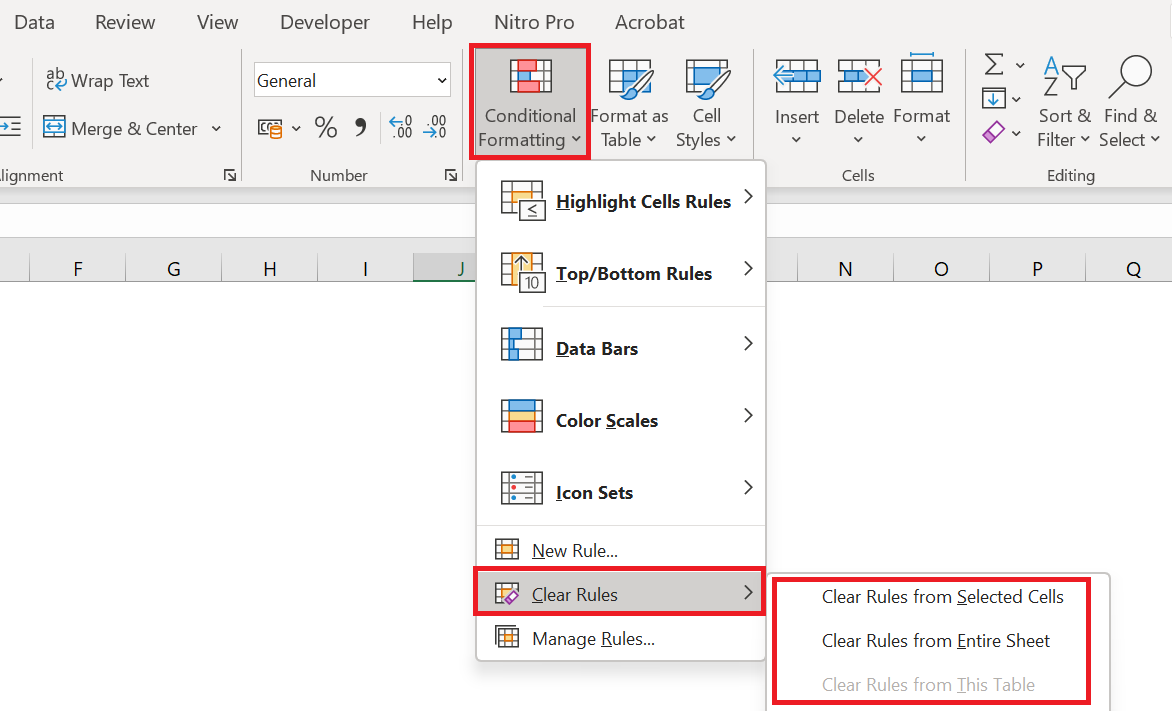
■ Clear Rules : Use these rules to remove all conditional formats you’ve created for a selected range or the entire worksheet.

■ Manage Rules : Use these rules to view, edit, and delete conditional formatting rules ; create new rules; or change the order in which Excel applies the conditional formatting rules you’ve defined.

2 Create conditional formatting rules

To truly take advantage of the capabilities of conditional formatting in Excel, you need to learn how to create different types of rules. This will help you understand the project you’re currently working on.

Conditional formatting rules in Excel define 2 key elements:

• Which cells should conditional formatting be applied to, and
• What conditions must be met.

We’ll show you how to apply conditional formatting in Excel. However, the options are essentially the same in all versions of Excel, so you’ll have no trouble following along no matter which version you have installed on your computer.

1. In your Excel spreadsheet, select the cells you want to format.

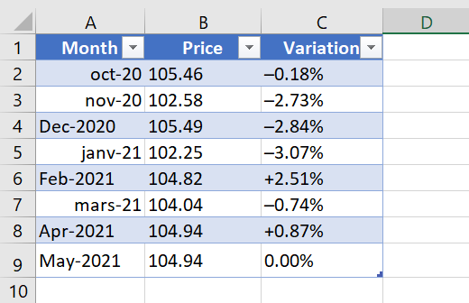
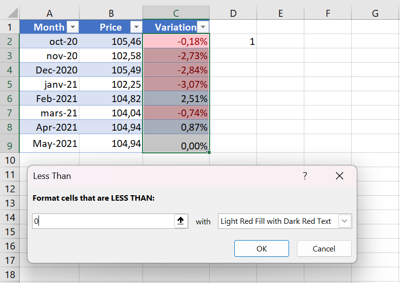
For this example, we’ve created a small table listing monthly crude oil prices. What we want is to highlight every price drop, that is, all cells with negative numbers in the Change column , so we select cells C2 : C9.

Go to the tab Home / Styles group and click Conditional Formatting . You’ll see several different formatting rules, including data bars, color scales, and icon sets.

1. Since we need to apply conditional formatting only to numbers less than 0, we choose Highlight Cell Rules / Less than …
   

Of course, you can go ahead with any other type of rule more appropriate for your data, such as:

• 1. Format values greater than, less than, or equal to
  2. Highlight text containing specified words or characters
  3. Highlight duplicates
  4. Format specific dates

1. Enter the value in the box on the right side of the window under  » Format cells less than « , in our case we type 0. As soon as you enter the value, Microsoft Excel will highlight the cells in the selected range that match your condition.
2. Select the desired format from the drop-down list. You can choose one of the predefined formats or click Custom Format … to configure your own formatting.
   
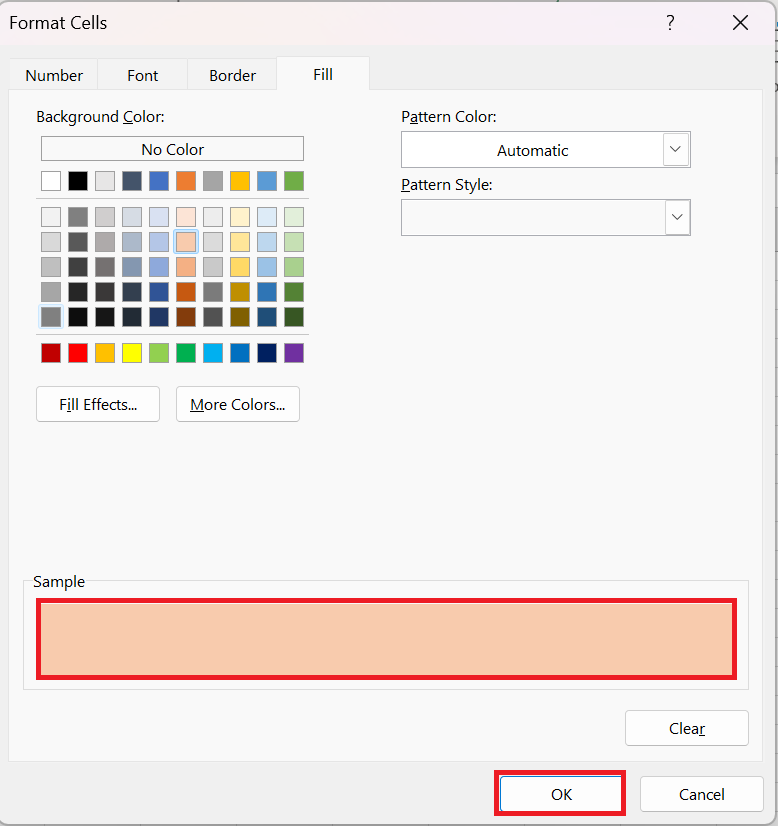
3. In the Format Cells window, switch between the Font, Border, and Fill tabs to choose the font style, border style, and background color, respectively. In the Font and Fill tabs, you’ll immediately see a preview of your custom format. When finished, click the OK button at the bottom of the window.

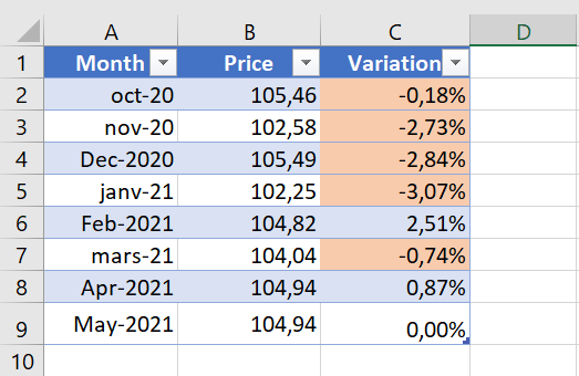
As you can see in the screenshot below, our new conditional formatting rule works correctly – it shades all cells with a negative price change.

3 Creating a Conditional Formatting Rule from Scratch

If none of the ready-made formatting rules meet your needs, you can create one from scratch.

1. Select the cells you want to apply the conditional format to and click Conditional Formatting / New Rule .

1. New Formatting Rule dialog box opens and you select the type of rule you want. For example, let’s choose  » Apply formatting only to cells that contain  » and choose to format the values in cells between 60 and 70 .

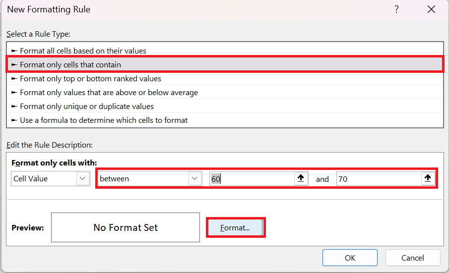
1. Click the Format… button and configure your formatting exactly as we did in the previous example.
2. OK twice to close any open windows and your conditional formatting is complete!

4 Conditional formatting based on cell value

In the previous two examples, we created the formatting rules by entering the numbers. However, in some cases, it makes more sense to base your conditional formatting on a specific cell value. The advantage of this approach is that, no matter how that cell’s value changes in the future, your conditional formatting will automatically adjust and reflect the changed data.

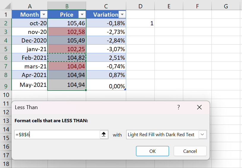
For example, let’s take the « Oil Price » example again, but this time highlight all prices in column B that are higher than the February price.

You create the rule in the same way by selecting Conditional Formatting / Highlight Cell Rules / Greater Than… But instead of typing a number in step 4, you select cell B6 by clicking the range selection icon as you usually do in Excel. As a result, the prices are formatted as you see in the screenshot below.

This is the simplest example of Excel conditional formatting based on another cell. Other, more complex scenarios may require the use of formulas. This is how you perform conditional formatting in Excel. Hopefully, these very simple rules we just created were helpful in understanding the general approach.

5 Apply multiple conditional formatting rules to a cell/table

When using conditional formatting in Excel, you’re not limited to a single rule per cell. You can apply as many rules as your project logic requires.

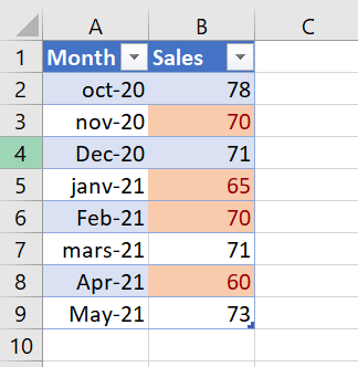
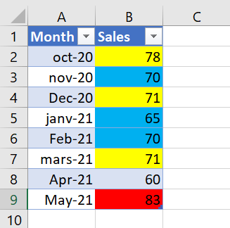
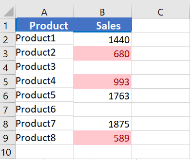
For example, let’s create 3 rules for the sales table that will shade sales above 60 in yellow, above 70 in orange, and above 80 in red.

You already know how to create Excel conditional formatting rules of this type – by clicking Conditional Formatting / Highlight Cell Rules / Greater Than . However, for the rules to work properly, you also need to set their priority like this:

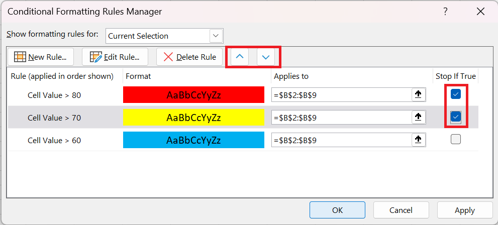
1. Click Conditional Formatting / Manage Rules… to display the Rules Manager .
2. Click on the rule that should be applied first to select it and move it up using the up arrow . Do the same for the second priority rule.
3. Check the Break if true box for the first 2 rules because you do not want the other rules to be applied when the first condition is met.

6 Using « Break if true » in conditional formatting rules

We have already used the Stop if true option in the example above to stop processing other rules when the first condition is met. This use is very obvious and straightforward. Now let’s consider two examples where the use of this function is not so obvious, but also very useful.

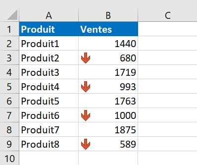
Example 1: Show only certain elements of the icon set

Let’s say you added the following icon set to your sales report.

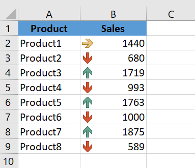
It looks nice, but a bit cluttered with graphics. So, our goal is to keep only the red downward arrows to draw attention to products with below-average performance and get rid of all the other icons. Let’s see how you can do this:

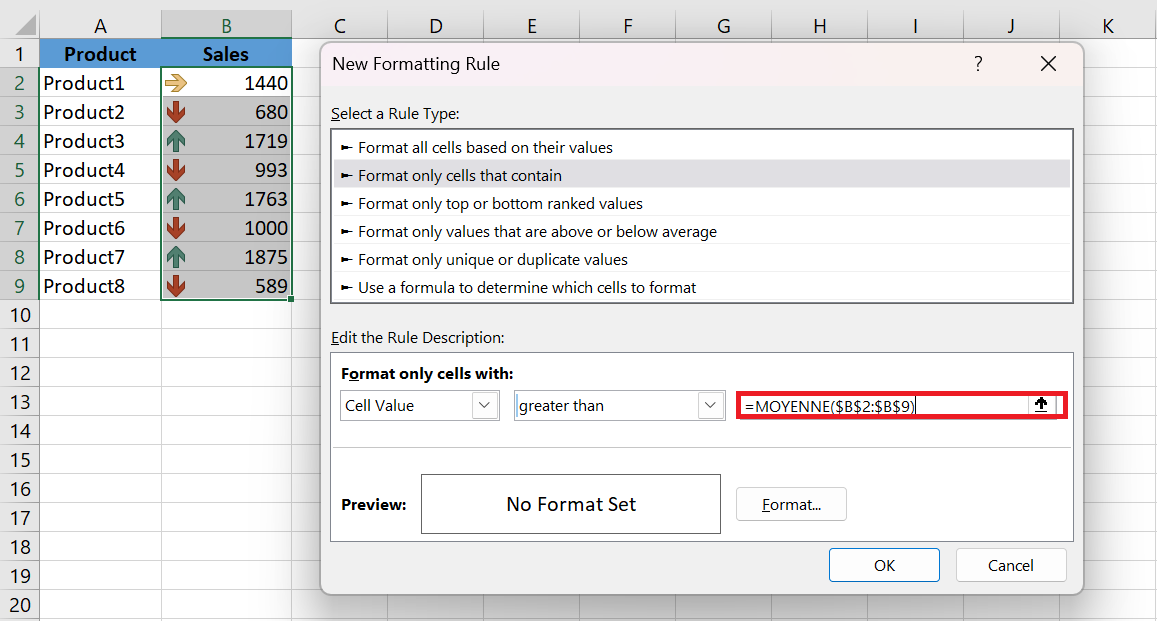
1. Create a new conditional formatting rule by clicking Conditional Formatting / New Rule / Apply Formatting only to cells that contain .
2. Now you need to configure the rule so that it only applies to values above the average. To do this, use the formula = AVERAGE( ) , as shown in the screenshot below.

You can still select a range of cells in Excel using the standard range selection icon or manually enter the range in parentheses. If you choose the latter, remember to use absolute cell references with the $ sign.

1. Click OK without setting a format.
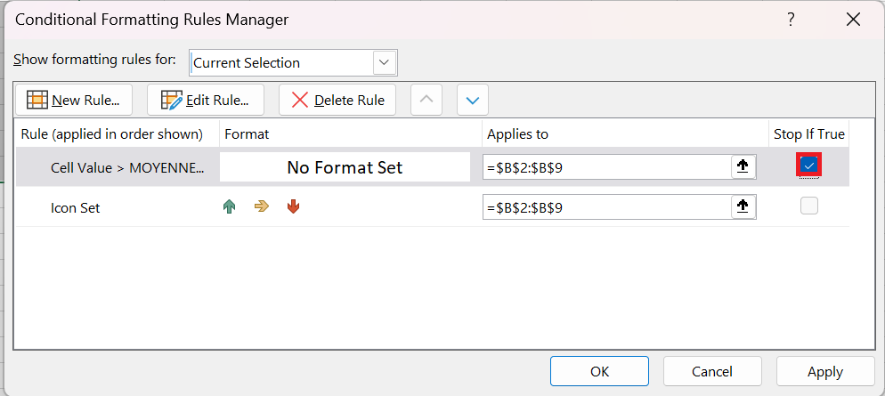
2. Click on Conditional Formatting / Manage Rules… and check the Break if True box for the rule you just created. And… see the result in the screenshot below : )

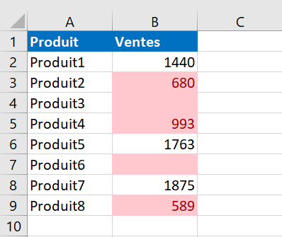
Example 2. Remove conditional formatting from empty cells

Let’s say you created the « Between » rule to highlight cell values between $0 and $1,000, as you can see in the screenshot below. But the problem is that empty cells are also highlighted.

To solve this problem, you create an additional rule of the type  » Apply formatting only to cells that contain « . In the New Formatting Rule dialog box , select Cells

empty in the drop-down list.

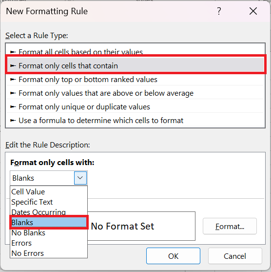
And again, you just click OK without setting any format.

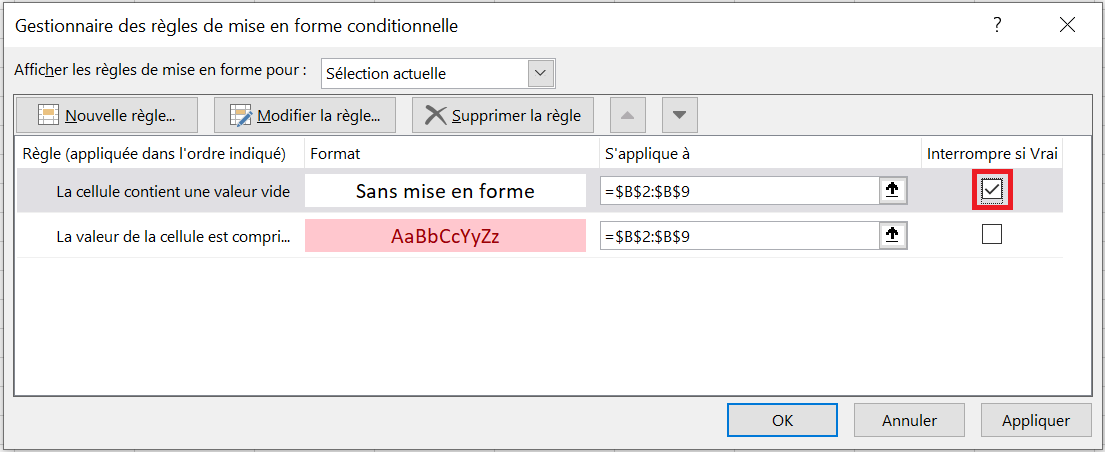
Finally, open the Conditional Formatting Rules Manager and check the Stop if true box next to the « Empty » rule.

The result is exactly as you would expect.

6 Edit conditional formatting rules

If you looked closely at the screenshot above, you probably noticed the Edit Rule… button there. So, if you want to edit an existing formatting rule, follow these steps:

1. Select any cell to which the rule applies and click Conditional Formatting / Manage Rules…
2. Formatting Rules Manager dialog box , click the rule you want to edit, and then click the Edit Rule… button.
   
3. Make the required changes in the Edit Formatting Rule window and click OK to save the changes.

Edit Formatting Rule window looks very similar to the New Formatting Rule dialog box you used when creating the rule, so you won’t have any trouble with it.

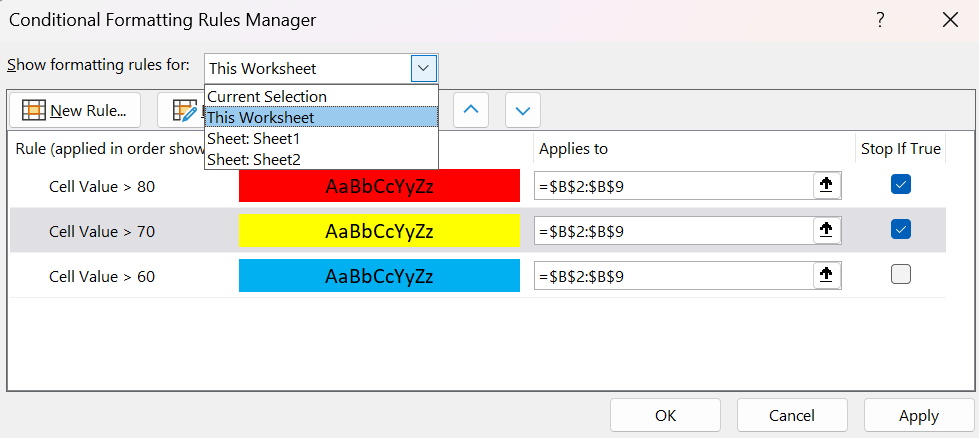
If you don’t see the rule you want to edit, select This worksheet from the  » Show formatting rules for  » drop-down list to display a list of all the rules in your worksheet.

7 Copy conditional formatting

If you want to apply the conditional format you created earlier to other data in your spreadsheet, you won’t need to create the rule from scratch. Simply use Format Painter to copy the existing conditional formatting to the new data set.

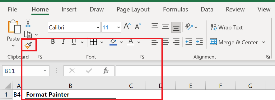
1. Click any cell with the conditional formatting you want to copy.
2. Click Home / Format Painter . This will change the mouse pointer to a paintbrush.

You can double-click Format Painter if you want to paste conditional formatting into multiple different cell ranges.

1. To paste conditional formatting, click the first cell and drag the brush to the last cell in the range you want to format.
2. When finished, press Esc to stop using the brush.

If you created the conditional formatting rule using a formula, you may need to adjust the cell references in the formula after copying the conditional formatting.

8 Delete conditional formatting rules

To delete a rule, you can either:

• Open the Conditional Manager Rules Manager (as you remember, you open it via Conditional Formatting / Manage Rules …) , select the rule and click the Delete Rule button.
• Select the cell range, click Conditional Formatting / Clear Rules and choose one of the available options.