Votre panier est actuellement vide !
Catégorie : Excel VBA Course
Assigning VBA Procedures to Buttons with Excel VBA
Now let us look at an example that allows you to run your VBA procedure directly from the Quick Access Toolbar.
Note that the sequence of steps to link a VBA procedure to a chosen button is similar to the one we followed when assigning a macro to a button.
Suppose we want to add four buttons to the Quick Access Toolbar, which will perform the following actions respectively:
- determine whether a given number of points with the center at the origin falls inside a circle,
- calculate employees’ commissions according to a certain rule,
- replace the values of cells in a selected range according to a specified rule,
- format numbers according to a specified rule.
Let us now consider in detail the conditions and the VBA procedures that implement the required actions.
The VBA procedure that determines whether a given number of points falls inside a circle centered at the origin is presented in the standard module Module1.
Next, here is an example of calculating employee commissions according to the following rule:
- if products are sold for 1,000,000 currency units or more, the commission is 4% of the sales value;
- if products are sold for less than 1,000,000 currency units, the commission is 2% of the sales value;
- if the employee has worked in the company for 5 years or more, an additional bonus of 1.5% of the sales value is paid.
The corresponding VBA procedure is written in the standard module Module2.
The standard module Module3 contains the procedure for replacing cell values in a selected range according to the following rule:
- positive numbers are replaced with « + »,
- negative numbers with « – »,
- zeros with « zero ».
In the standard module Module4, the procedure demonstrates formatting numbers in a selected worksheet range according to this rule:
- numbers from 0 to 1000 are formatted in red,
- numbers from 1000 to 10,000 are formatted in green,
- numbers above 10,000 are formatted in black,
- positive numbers use the data format #000,000,
- zeros are displayed in purple with the text « Zero!!! »,
- negative numbers are formatted in blue with the format #000,000.
So, to add buttons to the Quick Access Toolbar that perform the actions described above, follow these steps:
- Open the VBA editor by going to the Developer tab on the Ribbon, selecting the Code group, and clicking Visual Basic.
- In the VBA editor window, successively add 4 modules using the commands Insert | Module, and paste into each the corresponding VBA procedure code.
- Switch back to the Excel workbook window.
- Right-click the Quick Access Toolbar and select Customize Quick Access Toolbar.
- In the Excel Options window, in the Quick Access Toolbar category, choose Macros in the Choose commands from list.
- One by one, select your created procedures in the left column and transfer them to the right column using the Add button. Use the Modify button to change the icon for each button.
- After adding all your created procedures to the right column of the Excel Options – Quick Access Toolbar window, click OK.
- Make sure that the required buttons have appeared on the Quick Access Toolbar and that pressing them executes the actions you programmed.
Recording a Macro and Assigning It to a Button with Excel VBA
On the other hand, if you are developing your own application, you will of course need to create your own buttons that perform actions recorded with a macro or defined by a VBA procedure.
Let us look at an example that demonstrates how to record a macro and assign it to a button placed on the Quick Access Toolbar.
Suppose we need to create a macro that highlights the range A1:K20 on the active worksheet of an Excel workbook and applies the following formatting:
- Fill color — yellow
- Borders — all borders
- Font — Bookman Old Style, size 14 pt
- Font color — red
- Font style — bold
After performing these actions, the cursor should be set in cell A1.
So, open a Microsoft Office Excel 2010 workbook and make sure the cursor is in cell A1.
- Go to the Developer tab on the Ribbon and in the Code group, click Record Macro.
- In the Record Macro dialog box, set the required parameters for the procedure being recorded.
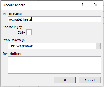
Remember that a macro name cannot contain spaces.
- While in recording mode, perform the required actions in this sequence:
- Go to the Home tab on the Ribbon and select the range A1:K20.
- Using the tools in the Font group on the Home tab, set the following: fill color — yellow; borders — all borders; font — Bookman Old Style; size — 14 pt; font color — red; font style — bold.
- Place the cursor back in cell A1.
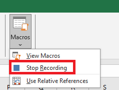
- Click Stop Recording in the Code group on the Developer tab to stop recording the macro.
- Save your workbook under the name Quick Access Toolbar Setup with Macros Enabled .
- Now switch, for example, to Sheet2 of your workbook.
- Click the Macros button in the Code group on the Developer tab.
- In the Macro dialog box,
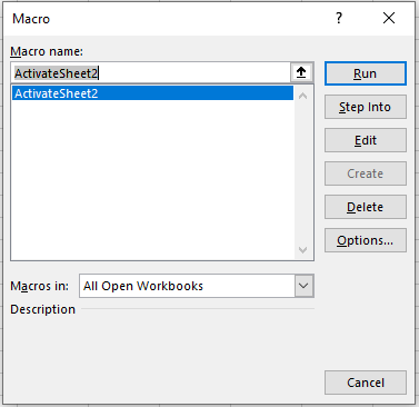
select the name of the macro you created and click Run. Verify that the macro performed all the necessary changes in your workbook .

Note
On the Developer tab, in the Code group, there is a Macro Security button, which opens the Trust Center window in the Macro Settings category.
You can always choose the required option to prevent the execution of malicious code that may be contained in macros from unknown sources.
Now let’s assign our created macro to a button on the Quick Access Toolbar.
- Right-click the Quick Access Toolbar and select Customize Quick Access Toolbar.
- In the Excel Options window, in the navigation pane, select the Quick Access Toolbar category, and in the Choose commands from drop-down list, choose Macros.
- In the left column, select the macro you created and click Add to move it to the right column. Notice that at the bottom of the right column the Modify button has become available: it is intended for assigning a button to the corresponding macro. Click Modify.
- In the Modify Button window, select a symbol for the button and type the desired display name for the macro, which will appear as a tooltip on the Quick Access Toolbar. C
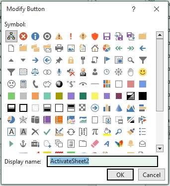
Click OK.
- In the Excel Options window, the button and new name for the macro appear in the right column.
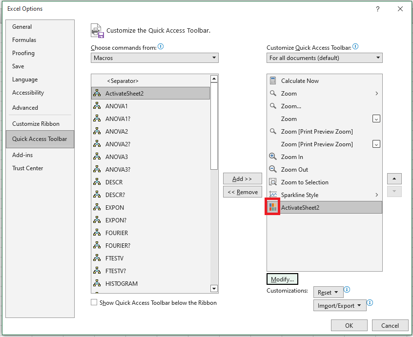
Click OK.
- Make sure that the button with the recorded macro now appears on the Quick Access Toolbar and that clicking it executes the actions you recorded.

How to Customize the Quick Access Toolbar with Excel VBA
Quite often, the Quick Access Toolbar is more convenient when performing calculations and formatting workbooks in Microsoft Office Excel 2010.
By default, it contains the following standard buttons: Save, Undo, Redo, and Customize Quick Access Toolbar.If you frequently use certain commands more than others, you can add the required button to the Quick Access Toolbar by clicking the Customize Quick Access Toolbar button and selecting either a command from the available list or the More Commands option.

In the latter case, the Excel Options window opens in the Quick Access Toolbar category, where you can choose the necessary buttons and add them to the toolbar using the options available in that window.

Another way to open the Excel Options window is as follows: click the File tab in Microsoft Office Excel 2010 and select the Options command. In the opened Excel Options window, go to the navigation pane and choose the Quick Access Toolbar category.
Note
Another method to open the Excel Options window in the Quick Access Toolbar category is to open the context menu of the Quick Access Toolbar and select Customize Quick Access Toolbar.Now you can add other buttons to the Quick Access Toolbar using the list boxes and control buttons: select a command from the left list and add it to the right list by clicking the Add button located between the two lists.
To remove a button from the Quick Access Toolbar, select it in the right column and use the Remove button (also located between the lists). The arrow buttons to the right of the right column allow you to adjust the order of the buttons on the Quick Access Toolbar.By default, only frequently used commands are displayed in the left pane. To change the list of commands, use the drop-down menu in the Choose commands from field and select the desired category: all commands, all commands on the ribbon, macros, commands from the Office menu (the menu that opens when you click the Microsoft Office button), or any ribbon tab.
When selecting a command from the Customize Quick Access Toolbar list, you can also specify where the added buttons will be used: only in the current workbook or in all Excel workbooks.
In addition to adding commands, in the Excel Options window under the Quick Access Toolbar category, you can also set the option to place the toolbar below the ribbon by checking the corresponding box at the bottom of the window.
The Settings group allows you to reset all Quick Access Toolbar settings or perform the appropriate import/export of settings.
Tip
To add any command from the ribbon to the Quick Access Toolbar, use the context menu: right-click the required ribbon button and select Add to Quick Access Toolbar.
The Customize Quick Access Toolbar option in the context menu also allows you to open the Quick Access Toolbar category of the Excel Options window.
To remove a button from the Quick Access Toolbar, open its context menu and choose Remove from Quick Access Toolbar.Developing a Warehouse Model with Excel VBA
The main steps for creating this application are as follows:
First, place the necessary data related to warehouse organization onto Excel worksheets:
- Create six sheets in the workbook: prod_pit, Storeage, shv_izd, aud_vid_texn, mebel, kanc_tov.
- On the Storeage sheet, place the service information required for the program’s operation (the number of product categories, the names of the product categories—food products, sewing items, audio/video equipment, furniture, office supplies—the number of items in stock for each category, the number of warehouse clerks, and their surnames).
- The other five sheets will store the actual data about the goods in the warehouse.
- For each type of product, the following information is stored: product name, weight/quantity, date of receipt into the warehouse, date of release from the warehouse, the warehouse clerk who accepted the goods, the clerk who released the goods, storage cost, and payment confirmation (yes/no).
Next, proceed to developing the main form of the warehouse application:
- Open the VBA code editor.
- Add a user form (via Insert | UserForm). Set the form’s Name property to MainForm.
- Place the necessary controls on the form and set their properties according to Table, so that they appear similar.
- Write code in the form module to handle events for the controls:
- From the drop-down list, select the product category.
- The corresponding goods stored on different worksheets will then appear in the list box below.
- The Receive Goods and Release Goods buttons should open forms that support the respective actions of receiving and releasing goods.

Table. Property values for MainForm and its controls set in the Properties window
Object Property Value Form Name MainForm Caption Warehouse Label Name Label1 Caption Goods Warehouse ComboBox Name ComboBox1 Style fmStyleDropDownList Button Name CommandButton1 Caption Receive Goods Button Name CommandButton2 Caption Release Goods ListBox Name ListBox1 BoundColumn 1 ColumnCount 1 ColumnHeads False The next step is to design the form for receiving goods and the form for releasing goods. The process here is similar to that used for developing the main form:
- configure the appropriate properties for the controls,
- and write the corresponding event-handling code.


Finally, place a button on the Storeage worksheet that opens the main form MainForm.
Also, make sure to enter the necessary code in the worksheet module to handle the button click.Filling a Tabular Data List with Excel VBA
One of the main advantages of MS Excel is its ability to work with homogeneous data arrays, called lists.
Lists in MS Excel are tables where rows contain uniform information.
The rows of the table are called records, and the columns are called fields of the records.Column fields are assigned unique names, which are placed in the first row of the list—the header row.
In Microsoft Office Excel 2010, for example, the following methods can be used to enter data into a list:
- Using the data form, which is automatically created after defining the list header with the Form command.
NOTE
In earlier versions of MS Excel (including 2003), the data form could be called using the menu command Data | Form.
In MS Excel 2007 and MS Excel 2010, you must add the corresponding Form command to the Quick Access Toolbar or to a ribbon tab by using the Excel Options window and selecting either Customize Ribbon or Quick Access Toolbar.- Entering data directly into empty rows inserted into the list (in this case, the list range name is automatically redefined).
- Using AutoFill, Series, and the Pick from List command to speed up work.
- Using MS Access forms and then transferring the data into an Excel worksheet.
- Using VBA—where a custom program you write provides a form or dialog box for data entry, which then inserts the values into specified worksheet cells.
The built-in Form tool, whose dialog box is displayed by choosing the Form command, allows filling and editing records in a table list.
A major drawback of this tool is that each field of a record corresponds only to a simple text box.
However, when filling list data, values for some fields are often chosen from a limited set of alternatives (e.g., gender can be male or female, the list of employees in a sales department is limited, etc.).
For such fields, it is more convenient to use list boxes, option buttons, and checkboxes instead of plain text fields.
This approach both speeds up the data entry process and reduces errors (typos) that inevitably occur during manual entry.
Example application
Let us create an application that eliminates the drawbacks of the standard form.Suppose you are a manager of a travel agency called Through Space and Time! and you are recording information about each client in a data list.
To speed up data entry, you decide to create an application with a dialog box.

To avoid mistakes, repetitive information such as tour destination and type of transport will be selected from lists.
These lists will be filled based on data stored in the worksheets Tour and Transport.Constructing the application
Create a form and place on it:- three text boxes,
- five labels,
- a spin button,
- two buttons,
- two combo boxes,
- one frame with two option buttons,
- and another frame with three checkboxes.
Using the Properties window, assign the properties shown in Table.
Table. Property values set in the Properties window
Object Property Value Form Caption Registration of tourists of “Through Space and Time!” Label Caption Last Name TextBox Name txtLName Label Caption First Name TextBox Name txtFName Frame Caption Payment and Documents CheckBox Caption Paid CheckBox Caption Photo CheckBox Caption Passport Label Caption Duration (days) TextBox Name txtDays SpinButton Name SpnDays Frame Caption Gender OptionButton Name optMale OptionButton Name optFemale Label Caption Destination (Tour) ComboBox Name cmbTour Label Caption Transport Type ComboBox Name cmbTrans Button Name cmdOK Button Name cmdCancel Form Module Functionality
In the form module, enter the necessary code, which provides:- Reading data from the dialog box and entering the record into the first empty row of the data table.
- Entering the duration of the tour either via the keyboard or the spin button, which work synchronously.
- Protecting all data on the worksheets from being modified by the user.
Additional Controls with Excel VBA
In VBA, in addition to the standard controls already listed, there are a number of additional controls.
These additional controls are independent objects that share the common properties and methods of all controls, while also having their own unique properties and methods.Adding an additional control
Additional controls can be added to the Toolbox (a new form must be added to the project) as follows:- Select the command Tools | Additional Controls.
- In the Additional Controls window that appears , check the box next to the control you want to add from the list of Available Controls.
- Click OK.

As a result, the icon for the selected additional control will appear in the Toolbox.
NOTE
When distributing an application that uses an additional control, you must include the corresponding OCX file. The name and location of the OCX file can be found in the Location field of the Additional Controls window.Removing an additional control
An unnecessary control can be removed from the Toolbox in almost the same way it was added:- Select the command Tools | Additional Controls.
- In the Additional Controls window that appears, uncheck the box next to the control you want to remove from the list of Available Controls.
- Click OK.
Displaying Built-in Dialog Boxes with Excel VBA
VBA allows you to programmatically display Excel’s built-in dialog boxes, in addition to user-defined dialog boxes. All built-in Excel dialog boxes form the Dialogs collection, where the parameter specifies which dialog box to activate.
Displaying a built-in dialog box on the screen is done using the Show method.
For example, the procedure activates the Open dialog box when a button is clicked.
Displaying the Open dialog box
Private Sub CommandButton1_Click()
    Application.Dialogs(xlDialogOpen).Show
End Sub
Table. Values of Dialogs collection parameter
Parameter Value Dialog Box xlDialogFindFile Open (file search) xlDialogFileDelete Delete file xlDialogGoalSeek Goal Seek xlDialogSaveAs Save As xlDialogSaveWorkbook Save xlDialogPrint Print xlDialogPrintPreview Print Preview 
Within the Show method, you can specify parameter values that prefill fields in the dialog box.
For example, when displaying the Goal Seek dialog box, you can specify:
- target_cell (Set Cell field),
- target_value (To Value field),
- variable_cell (By Changing Cell field).
This results in the dialog box appearing with its input fields already filled.
Displaying Goal Seek with predefined values
Private Sub DoGoalSeek()
    Dim fl As Boolean
    fl = Application.Dialogs(xlDialogGoalSeek).Show(Range("A1"), 0, Range("A2"))
    If fl Then
        MsgBox "Solution found"
    Else
        MsgBox "Solution not found"
    End If
End Sub
Open Dialog and the GetOpenFilename Method
There is another way to display the Open dialog box—using the GetOpenFilename method of the Application object.This method displays the Open dialog box, but it does not open the selected file. Instead, it simply returns the name of the selected file, or the value False if no file was selected.
To open the selected file, you must additionally use the Open method of the Workbooks collection.
Opening a file
Sub OpenDoc()
    Dim FName As Variant
    FName = Application.GetOpenFilename( _
        "Microsoft Excel Workbook (*.xlsx), *.xlx")
    If FName <> False Then
        Workbooks.Open FName
    Else
        MsgBox "No file selected"
    End If
End Sub
The appearance of the dialog box can be controlled by setting parameters of the GetOpenFilename method.
Syntax:
GetOpenFilename(FileFilter, FilterIndex, Title, ButtonText, MultiSelect)
- FileFilter — Optional. A string specifying the filter for displayed files. If omitted, defaults to « All files (*.*), *.* ».
Example: « Microsoft Excel Workbook (*.xlsx), *.xlsx, Bitmap Files (*.bmp), *.bmp ». - FilterIndex — Optional. Sets which filter index is used by default.
- Title — Optional. Sets the title of the dialog box.
- ButtonText — Used only in Mac OS X.
- MultiSelect — Optional. Boolean. If True, allows selection of multiple files. In that case, the method returns an array of file names instead of a single string.
Since GetOpenFilename only returns file names (without acting on them), the dialog box can also be used for purposes other than opening files—for example, deleting selected files.
Deleting files
Sub DeleteFile()
    Dim FName As Variant
    FName = Application.GetOpenFilename( _
        FileFilter:="Microsoft Excel Workbook (*.xls), *.xls", _
        MultiSelect:=True, Title:="Delete File")
    If Not IsArray(FName) Then
        MsgBox "No file selected"
        Exit Sub
    End If
    Dim i As Integer
    For i = LBound(FName) To UBound(FName)
        Kill FName(i)
    Next
End Sub
A Simple Graphic File Browser
The GetOpenFilename method returns the name of any type of file, including bitmap files.
At the same time, an Image control can display any bitmap file.Together, these two facts make it possible to create a simple tool for browsing bitmap images.
So, create a form with a button and an Image control, and in the form module type the necessary code.
The project is ready.

Saving a Document and the GetSaveAsFilename Method
The GetSaveAsFilename method of the Application object displays the Save As dialog box.Like the GetOpenFilename method, this method does not itself save the file—it only returns the name of the file chosen in the dialog box.
To actually save the file, you must extend the code with a statement that uses either the SaveAs or Save method of the Workbook object.Syntax
GetSaveAsFilename(InitialFilename, FileFilter, FilterIndex, Title, ButtonText)
- InitialFilename — Optional. Any valid file name that will appear in the File name field. (By default, Excel suggests the name Book.)
- FileFilter — Optional. Sets the filter for the displayed files. If you want a file extension to be automatically added to the file name, this parameter must be used.
- FilterIndex — Optional. Indicates which filter from the File types list will be used by default.
- Title — Optional. Sets the dialog box title.
- ButtonText — Used only in Mac OS X.
Example
The following code can be used when saving a workbook, where by default the suggested file name is Report.Saving a file
Sub SaveDoc()
    Dim FName As Variant
    FName = Application.GetSaveAsFilename(InitialFilename:="Report", _
        FileFilter:="Microsoft Excel Workbook (*.xlsx), *.xls")
    If FName <> False Then Application.ThisWorkbook.SaveAs FName
End Sub
MultiPage and TabStrip with Excel VBA
The MultiPage control allows you to create multi-page dialog boxes. Page titles are displayed on tabs. Navigation between pages is done by clicking a tab.
You can create, rename, delete, or move a page of the MultiPage control manually by right-clicking the tab label and using the context menu.
The MultiPage object contains the Pages collection, which represents all the pages included in this object.
Table lists the main properties of the MultiPage object.Table. Main properties of MultiPage
Property Description Value Returns or sets the index of the active page. Indexing starts at 0. MultiRow A Boolean property. If set to True, tab labels that do not fit in one row are displayed in multiple rows. If set to False, a scrollbar appears when tab labels do not fit in one row, allowing navigation between pages. SelectedItem Returns the selected page. The Pages collection consists of all Page objects, i.e., the pages of a MultiPage control.
The Pages collection has only one property, Count, which returns the number of elements in the collection.
Its methods are listed in Table.Table. Methods of the Pages collection
Method Description Add Creates a new page. Clear Deletes all pages from the collection. Remove Deletes a page from the collection. Item Returns the page specified by index. The TabStrip control creates multiple tabs in a dialog box and is functionally equivalent to a MultiPage control.
The TabStrip object contains the Tabs collection, which represents all the tabs.The TabStrip object and the Tabs collection have the same properties and methods as the MultiPage object and the Pages collection.
Statistics and MultiPage
As an example of an application with multiple pages, let us improve the interface of the project from the earlier section “Determining statistical parameters of a range” .Create a form with a MultiPage control:
- On the first page (set the Caption property to Calculations), place a RefEdit control, a text box, and a button.
- On the second page (set the Caption property to Parameters), place three checkboxes.
Use the Properties window to set the control properties as shown in Table.
Table. Property values set in the Properties window
Object Property Value TextBox Name txtStat Button Name cmdOK Caption OK CheckBox Name chkSum Caption Sum CheckBox Name chkMax Caption Maximum CheckBox Name chkMin Caption Minimum In the form module, type the required code. The project is ready.
The text box displays multi-line integrated statistics, with the parameters determined by the checkboxes on the Parameters page.
The text box is locked to prevent the user from editing the results.
In addition, the background color of the text box is set equal to the form’s background color.As a result, the text box visually appears as an indented label within the form.

RefEdit Controlwith Excel VBA
The RefEdit control is similar to a text box, but it allows you to enter a reference to a range by selecting it directly on the worksheet.
The Value property returns this reference.TIP
To add the RefEdit control to the Toolbox panel, right-click on the panel and select Additional Controls. In the Additional Controls window that appears, select RefEditCtrl from the list of available controls and click OK.Determining statistical parameters of a range
As an example of using the RefEdit control, let us construct a simple project that determines some statistical parameters of a range—namely, the maximum, minimum, and the sum of all cell values in that range.So, create a form with a button and a RefEdit control.
In the form module, type the necessary code.The project is ready.
To calculate the maximum, minimum, and sum of all values in the range, we use the Max, Min, and Sum properties of the WorksheetFunction object, which correspond to the worksheet functions of the same name.

Solving a system of linear equations
As another example of using the RefEdit control, let us create a project for solving systems of linear equations AX = B.Here:
- A is an n × n square matrix (the coefficients),
- B is the column of constants,
- X is the column of unknowns.
To solve the system of equations, we use the worksheet functions MInverse() (МОБР in Russian Excel) and MMult() (МУМНОЖ in Russian Excel), which return the inverse of a given matrix and the result of multiplying two matrices, respectively.
Additionally, the MDeterminant() (МОПР in Russian Excel) function is used to check whether the system has a solution by calculating the determinant of the coefficient matrix.
The form window contains a RefEdit control and a button.
The user enters into the RefEdit control a reference to a range of size n × (n+1), where the first n columns contain the coefficient matrix and the last column contains the constants.
Clicking the button triggers the calculation of the solution, which is then output into the range immediately to the right of the selected one.
For example the following system of linear equations is solved:
- The coefficient matrix is in range B3:C4.
- The column of constants is in range D3:D4.
- The solution of the system is displayed in range E3:E4.

Slide show with Excel VBA
The Image control allows you to create a simple slide viewer.
As a demonstration, let us create an application for viewing several images.
Create a form with an Image control and a list. In addition, you will need files with corresponding raster images.
In the form module, enter the required code. That’s all — the project is ready.

Modified Chart Wizard
Building a chart with the Chart Wizard normally requires a large amount of preparatory work:- filling one range with argument values,
- filling another range with function values,
- and then building the chart through a four-step wizard.
Let us create an application that will fill the ranges with argument and function values, build the chart, and display it not only on the worksheet but also in a form.
In this application, the user will only need to enter the interval boundaries and the function itself. The function should be entered not as a worksheet formula but in the usual form, using the symbol « z » as its argument.
The use of « z » as the argument is intended to simplify the code.
Constructing the application
Create a form with three labels, three text boxes, an image, and a button.
Set their Name properties in the Properties window as shown in Table.Table. Property values of controls set in the Properties window
Control Name Description TextBox txtBegin Input of the left boundary of the interval Label lblBegin Label corresponding to txtBegin TextBox txtEnd Input of the right boundary of the interval Label lblEnd Label corresponding to txtEnd TextBox txtFun Input of the function formula. The formula must follow programming rules, with « z » as the argument. Label lblFun Label corresponding to txtFun Image imgFun Displays a raster image from Graph.gif, which contains the graphic representation of the chart. Button cmdReady Triggers the building of the chart. How the application works
The chart is built from 101 points. First, the step size of the argument is calculated as the difference between the start and end values divided by 100.The initial argument value is placed in cell A2.
Using the DataSeries method, the argument values are tabulated down the column.In the function formula, the argument « z » is replaced with a reference to cell A2, and the formula is prefixed with the equals sign « = ».
This formula is entered into cell B2.
With the AutoFill method, the formula is filled down the column to compute the function values for all tabulated arguments.Based on the argument and function values, a chart is built, and its graphic representation is exported to the file Graph.gif.
The raster image from Graph.gif is then displayed in the Image control imgFun.
Why “z” is used as the argument
Using « z » as the parameter makes the code simpler, since « z » is not part of any built-in worksheet function names.Thus, it is sufficient to use the single instruction:
f = Replace(LCase(f), « z », « A2 »)
This replaces all occurrences of « z » with the reference to cell A2.
If « x » were used instead, one instruction would not be enough, because « x » appears in built-in function names (for example, Exp()).
In such a case, the instruction would replace not only the argument but also parts of function names, turning Exp() into EA2p(), which would result in an error.