Votre panier est actuellement vide !
Étiquette : Information
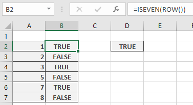
How to use the ISEVEN function in Excel
This function returns TRUE if the number is even, and FALSE if it is odd.
Syntax
ISEVEN(number)
Arguments
- number (required) – The expression to be checked.
Background
- Accepts any numeric expression.
- Integers are evaluated directly.
- Decimal numbers are truncated before evaluation (e.g., 2.4 becomes 2, -1.6 becomes -1).
- Returns #VALUE! for non-numeric inputs (e.g., text, logical values).
- Counterpart to ISODD():
ISEVEN(number) = NOT(ISODD(number))
Example
Scenario: Apply alternating row colours in a worksheet using conditional formatting.
- Preferred Method:
Use ISEVEN() with the ROW() function:
=ISEVEN(ROW())
-
- Applies formatting to even-numbered rows
- How it works: Divides the row number by 2 and compares the truncated result to the original division. If equal, the row is even.
How to use the ISERROR function in Excel
This function returns TRUE if the value is any error value (including #N/A). Otherwise, it returns FALSE.
- Unlike ISERR(), this function does recognize #N/A as an error.
Syntax
ISERROR(value)
Arguments
- value (required) – The expression to check (a number, text, a formula without an equal sign, a logical value, an error value, a reference, or a name).
Background
- Part of the IS() function family, which returns a logical value based on the argument.
- The input is not converted during evaluation (e.g., a numeric string remains text).
- Often paired with IF() to validate calculations before processing.
- Useful for conditional formatting and data validation rules.
- For detailed error identification, see ERROR.TYPE() examples.
Example
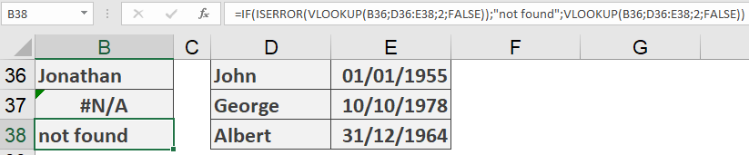
Suppose you use VLOOKUP() to search a list (e.g., birthdays, order numbers, or contact details).
- Problem:
Entering =VLOOKUP(B36; D36:E38; 2; FALSE) in B37 returns #N/A if no match exists—undesirable in printed reports. - Solution:
Replace the formula in B38 with:
=IF(ISERROR(VLOOKUP(B36; D36:E38; 2; FALSE)); « not found »; VLOOKUP(B36; D36:E38; 2; FALSE))
-
- If VLOOKUP() results in any error (including #N/A), it displays « not found ».
- Otherwise, it returns the lookup result.
Note: Adjust the delimiter (comma/semicolon) based on your Excel regional settings.
How to use the ISERR function in Excel
This function returns TRUE if the value is an error value. Otherwise, it returns FALSE.
- Exception: Unlike ISERROR(), this function does not recognize #N/A as an error and returns FALSE for it.
Syntax
ISERR(value)
Arguments
- value (required) – The expression (a number, text, a formula without an equal sign, a logical value, an error value, a reference, or a name) that you want to check.
Background
This function is one of the nine IS() functions that return a logical value based on the argument. The argument in IS() functions is not converted for evaluation—meaning a numeric string is treated as text, not a number.
IS() functions are often used with IF() to pre-test calculations. Their results can also be used in conditional formatting and data validation rules.
For more on identifying specific errors, see the ERROR.TYPE() function examples.
Example
Suppose you want to calculate the average of a range (B26:B28) while avoiding errors if no numbers are present.
=IF(ISERR(AVERAGE(B26:B28)); « Check the input values. »; AVERAGE(B26:B28))
IMAGE ISERR
- If AVERAGE(B26:B28) results in an error (except #N/A), the formula returns « Check the input values. »
- Otherwise, it returns the calculated average.
How to use the ISBLANK function in Excel
This function returns TRUE if the value argument refers to an empty cell. Otherwise, it returns FALSE.
Syntax
ISBLANK(value)
Arguments
- value (required) – The expression (a number, text, a formula without an equal sign, a logical value, an error value, a reference, or a name) that you want to check.
Background
This function is one of the nine IS() functions that return a logical value based on the argument. The argument in IS() functions is not converted for evaluation. This means that a string representing a number is treated as text, not as a numeric value.
IS() functions are often used with the IF() function to pre-test calculation results. The output of an IS() function can also be used in conditional formatting and data validation rules.
The function returns FALSE not only for non-empty cell references but also for arguments that are not valid references (e.g., text, numbers, logical values, or errors).
Example
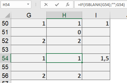
Using cell references to display values can sometimes produce unexpected results. In Figure below, column H contains references to cells in column G. Rows 50–52 use =G50, =G51, and =G52, and column I calculates the average of the three numbers in column H (0, 1, 2). However, this is incorrect because column G does not contain the number 0—it has a blank cell.
The correct solution is shown in rows 54–56. Here, the values in column H are pre-tested for blank cells, avoiding the assumption that a blank entry equals 0. The formula used is:
=IF(ISBLANK(G54); « »; G54)
How to use the ERROR.TYPE function in Excel
This function returns a number corresponding to an error value in Excel. If no error exists in the cell or in the calculation, the function returns the #N/A error.
Syntax
ERROR.TYPE(error_value)
Arguments
- error_value (required) – The error value (either the actual error in a cell or the result of a calculation) for which you want to find the error code.
Background
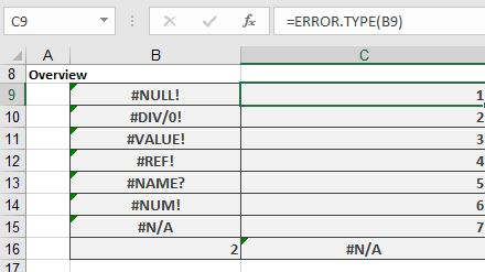
You can use this function in an IF() function to replace an error value with a descriptive string. To do this, you need to know the relationship between error values and their corresponding return codes (see Table 1).
Table 1. Error Values and Results of the ERROR.TYPE Function
Error Value Return Value #NULL! 1 #DIV/0! 2 #VALUE! 3 #REF! 4 #NAME? 5 #NUM! 6 #N/A 7 No error #N/A Examples
The following examples illustrate how to use the ERROR.TYPE() function.
- Conditional Formatting
Assume you want to use conditional formatting to highlight cells with errors in different colors.
- Figure below shows an example using the ISERROR() function to highlight error cells in a user-defined color.
- A critical error (e.g., division by zero, where ERROR.TYPE() returns 2) can be highlighted in a second color (e.g., red).
Note: Pay attention to the order of conditions. If ISERROR() is checked first, a specific error check (like #DIV/0!) may be ignored.
- Custom Functions
If you frequently need to map error types (1–7) to their descriptions (e.g., #DIV/0!), you can create a custom function for efficiency.
The following VBA code provides a solution:
Function ErrorDescription(Range As Range)
If WorksheetFunction.IsError(Range.Value) Then
Select Case CStr(Range.Value)
Case « Error 2000 »
ErrorDescription = « Intersection is empty »
Case « Error 2007 »
ErrorDescription = « Division by zero »
Case « Error 2015 »
ErrorDescription = « Noncalculable expression »
Case « Error 2023 »
ErrorDescription = « Lost reference »
Case « Error 2029 »
ErrorDescription = « Name not defined »
Case « Error 2036 »
ErrorDescription = « Number cannot be shown »
Case « Error 2042 »
ErrorDescription = « Nonexistent value »
End Select
Else
ErrorDescription = « No error »
End If
End Function
How to use the CELL function in Excel
This function retrieves details about the formatting, location, or contents of the upper-left cell in a specified range.
Syntax
CELL(info_type;[reference])
Arguments
- info_type (required)
A text string specifying the type of information to return (see in table 1). - reference (optional)
The cell being analyzed. If omitted, the function returns data for the last modified cell.
Background
The CELL() function requires knowledge of valid info_type arguments (listed below). Some return values are encoded (see Table 2 for number formats).
Table 1. info_type Arguments and Return Values
Argument Returns « address » Absolute reference of the cell (e.g., « $A$1 »). Includes sheet name if workbook is open. « width » Column width (rounded to integer), measured in characters of the default font. « filename » Full file path (empty if unsaved). « color » 1 if cell formats negative values in color; otherwise 0. « format » Text code for the cell’s number format (see Table 11-3). Appends « – » for color-negative or « () » for parentheses. « contents » Cell value (ignores formulas). « parentheses » 1 if cell uses parentheses for positives/all values; otherwise 0. « prefix » Text alignment marker: ‘ (left), » (right), ^ (center), \ (fill), or « » (other). « protect » 1 if cell is locked; 0 if unlocked. « col » Column number (e.g., 2 for column B). « type » Data type: « b » (blank), « l » (text), « v » (other). « row » Row number (e.g., 5 for row 5). Table 2. Number Format Codes
CELL() Returns Meaning « G » General « F0 » 0 « 0 » #,##0 « F2 » 0.00 « ,2 » #,##0.00 « C0 » Currency (no decimals) « C0-« Currency (no decimals, negatives in red) « C2 » Currency (2 decimals) « C2-« Currency (2 decimals, negatives in red) « P0 » 0% « P2 » 0.00% « S2 » Scientific (e.g., 0.00E+00) « D1 » Date: MM.DD.YY « D2 » Date: MM.DD « D3 » Date: MM.YY « D4 » Date: DD/MM/YY « D5 » Date: DD/MM « D6 » Time: h:mm:ss AM/PM « D7 » Time: h:mm AM/PM « D8 » Time: h:mm:ss « D9 » Time: h:mm Examples
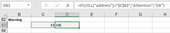
- Track Cell Changes
- Display a warning if C63 is modified:
=IF(CELL(« address »)= »$C$63″, « Caution », « OK »)
-
- Highlight the changed cell directly (using conditional formatting):
=(CELL(« address »)= »$C$63″)
- Note: Resets when another cell is edited.
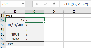
- Simplify Repeated Use
- Store info_type in a cell (e.g., B51 = « type »):
=CELL($B$51; B52) // Instead of =CELL(« type »;B52)
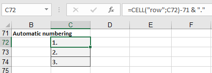
- Generate Consecutive Numbers
- Start numbering from row 72
=CELL(« row »; C72) – 71 & « . »
Result: 1., 2., etc.
Practical Tips
- IntelliSense aids formula entry.
- Conditional Formatting: Use CELL(« protect », …) to color-code locked/editable cells.
- Dynamic References: Combine with INDIRECT() for flexible lookups.
- info_type (required)