Votre panier est actuellement vide !
Étiquette : Information
How to use the TYPE function in Excel
This function returns a number indicating the data type of the specified value.
Syntax: TYPE(value)
Arguments:
- value (required): The expression to check (a number, text, a formula without an equal sign, a logical value, an error value, a reference, or a name).
Background:
- The TYPE() function is related to the IS() functions, which return logical values based on the argument’s type.
- It is often used with IF() to pre-test calculation results, and its output can support conditional formatting and data validation rules.
- To use this function effectively, refer to the mappings in Table 1.
Table 1. Data Types Mapped to Numbers
Argument Return Value Number 1 Text 2 Logical value 4 Error value 16 Array 64 Key Notes:
- Except for arrays, the results can also be obtained using ISNUMBER(), ISTEXT(), ISNONTEXT(), ISLOGICAL(), and ISERROR(). For example:
- ISNUMBER(B12) and TYPE(B12) = 1 are logically equivalent.
- Limitations:
- ISBLANK(), ISNA(), ISREF(), and ISERR() (which excludes #N/A) are incompatible with TYPE().
- TYPE() cannot detect whether a cell contains a formula—it only returns the result’s data type.
- For array formulas, TYPE() returns 64 only if the argument is a range entered with Ctrl+Shift+Enter.
Examples:
- Replicating IS() Functions:
- Replace =ISERROR(B3) with =(TYPE(B3)=16).
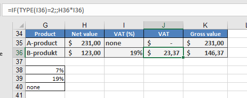
- Replace =IF(ISTEXT(I36);;H36*I36) with =IF(TYPE(I36)=2;;H36*I36).
How to use the NA function in Excel
This function returns the #N/A error value, indicating that a value does not exist.
Syntax: NA
Arguments:
- This function does not take any arguments.
Background:
- Although the NA() function does not require arguments, you must include the parentheses; otherwise, Excel will interpret it as text.
- Similar to TRUE() and FALSE(), where you can directly enter logical values (TRUE or FALSE), you can also manually enter #N/A instead of using NA() to achieve the same result.
- This function is primarily included for compatibility with other spreadsheet applications.
Usage Notes:
- You can use NA() (or #N/A) to explicitly mark empty cells, ensuring they are excluded from calculations.
- However, formulas referencing cells containing #N/A will also return the error, so use this function with caution.
Example:
- In the example for the ISBLANK() function, empty cells were checked to exclude them from calculations. If NA() were used instead, the desired result would not be obtained.
- Scenario:
- Column C references Column B, and the average is calculated in cell D2.
- If C3 contained a 0, it would not match Column B, so the empty cell in B is marked as =NA() or #N/A.
- However, the #N/A error propagates into all calculations.
Workaround:
=IF(ISNA(B7), « », B7)
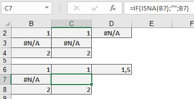
This formula returns the correct result, similar to what the ISBLANK() function would provide.
How to use the N FUNCTION in Excel
This function returns a value converted into a number.
Syntax. N(value)
Arguments
- value (required). The expression (a number, text, a formula without an equal sign, a logical value, an error value, a reference, or a name) that you want to convert into a number.
Background. Usually, you don’t need to use the N() function because Excel automatically converts values when a number is required. However, the IS() functions are an exception. For compatibility with other spreadsheet software, this function remains available.
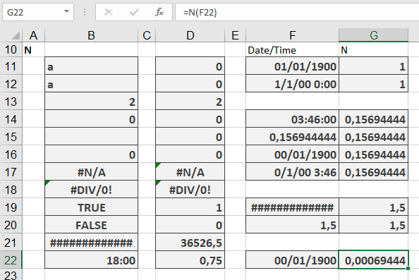
The N() function converts expressions as shown in Table 1.
Table 1. Conversion Results with the N() Function
Argument (Expression) Return Value Number The same number Date Serial number for the date Time Number for the time TRUE 1 FALSE 0 Error value The same error value Text or an empty cell 0 Example. For examples of this function’s usage, see the « Time Basics » Inside Out sidebar in this chapter.
How to use the ISTEXT function in Excel
Returns TRUE if the value is text (including numeric strings like « 123 »). Returns FALSE for numbers, errors, logical values, empty cells, or empty strings (« »).
Syntax
ISTEXT(value)
Key Behavior
Input Type ISTEXT Result Notes Regular text TRUE « Apple », « 123 » Empty cell FALSE Number FALSE 100, 3.14 Boolean FALSE TRUE/FALSE Error FALSE #N/A, #VALUE! Empty string (« ») FALSE Result of formulas like = » » Practical Applications
- Sales Tax Calculation (Text vs. Number)
Scenario: Column M contains either text (e.g., « Exempt ») or tax rates (e.g., 7%).
=IF(ISTEXT(M42); « »; L42*M42)
- Text in M42 → Returns blank (« »)
- Number in M42 → Calculates L42*M42
- Data Validation (Text-Only Fields)
Restrict cell input to text:
- Select cell → Data → Data Validation → Custom
- Formula:
=ISTEXT(A1)
- Clean Mixed Data
Identify text entries in a column:
=IF(ISTEXT(B2), « Text », « Not Text »)
Special Notes
- Numeric Strings:
- ISTEXT(« 100 ») → TRUE
- ISTEXT(100) → FALSE
- Empty vs. Zero:
- Blank cell → FALSE
- Formula returning « » → FALSE
- Counterpart:
ISTEXT(value) = NOT(ISNONTEXT(value))
Example Walkthrough
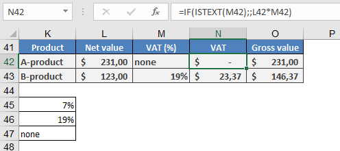
Problem: Calculate gross values where tax rates may be text (« Exempt ») or numbers (7%, 19%).
Solution:
=IF(ISTEXT(M42); ; L42*M42)
- If M42 is « Exempt » → Skips calculation (returns blank)
- If M42 is 0.07 (7%) → Multiplies by L42

Data Validation Setup:
- Create a list of valid inputs (e.g., « Exempt », 7%, 19%) in another sheet (e.g., column K).
- Apply to column M:
- Data → Data Validation → List
- Source: =$K$1:$K$3
Pro Tip
Combine with TRIM() to handle spaces:
=ISTEXT(TRIM(A1)) // Returns FALSE for cells with only spaces
How to use the ISREF function in Excel
Returns TRUE if the value is a valid cell reference (including named ranges). Returns FALSE for all other inputs (numbers, text, invalid references).
Syntax
ISREF(value)
Key Features
What Returns TRUE?
✔ Standard references (A1, Sheet2!B5)
✔ Named ranges (« Sales Data »)
✔ Structured references (Table1[Column1])What Returns FALSE?
✖ Numbers/text (123, « A1 »)
✖ Formulas (SUM(A1:A10))
✖ Invalid references (-B1, XYZ!A1 for non-existent sheets)Special Cases
⚠ Returns TRUE for references to non-existent sheets/tables (e.g., SheetX!A1), as Excel only validates syntax, not existence.
Practical Applications
- Safeguarding Named Ranges
Prevent #NAME? errors when a named range might be deleted:
=IF(ISREF(ABC), AVERAGE(ABC), « Error: Named range ‘ABC’ was deleted »)
- Dynamic Formula Validation
Check if a cell contains a valid reference before using:
=IF(ISREF(INDIRECT(B1)), « Valid reference », « Invalid input »)
- Conditional Formatting
Highlight cells containing references:
=ISREF(A1) // Applies formatting to reference-containing cells
Example Breakdown
Scenario
A workbook uses a named range ABC for calculations. To avoid #NAME? errors if ABC is deleted:
Original (Risky):
=AVERAGE(ABC) // Fails with #NAME? if ABC is deleted
Protected Version:
=IF(ISREF(ABC), AVERAGE(ABC), « removed Named ABC « )
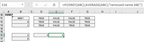
Behaviour:
- If ABC exists → Returns average
- If ABC is deleted → Shows friendly message
Limitations
- Cannot detect circular references or broken links.
- Returns TRUE for syntactically valid but non-existent references (e.g., Sheet99!A1).
For robust reference checking, combine with other functions like IFERROR() or ISERROR().
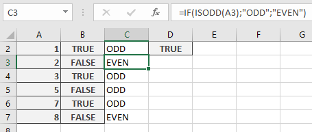
How to use the ISODD function in Excel
Its returns TRUE if the number is odd, and FALSE if it is even.
Syntax
ISODD(number)
Arguments
- number (required) – The value to check (can be a cell reference, formula, or direct input).
Key Behavior
✅ Integers: Evaluates normally (e.g., 3 → TRUE, 4 → FALSE).
Decimals: Truncates decimal places before checking (e.g., 5.9 → TRUE, -2.3 → FALSE).
❌ Non-numbers: Returns #VALUE! for text/logical values (e.g., « ABC », TRUE).
Counterpart: ISODD(number) = NOT(ISEVEN(number)).Practical Examples
- Conditional Formatting for Odd Rows
Goal: Shade every odd-numbered row.
=ISODD(ROW())
Data Categorization
Label numbers as odd/even:
=IF(ISODD(A3), « Odd », « Even »)
Notes
⚠️ Add-In Requirement: In Excel, ISODD() requires the Analysis ToolPak. The workaround avoids this.
Alternate Formula: For compatibility, use modulo:=MOD(TRUNC(A1), 2) = 1
How to use the ISNUMBER function in Excel
Returns TRUE if the value is a numeric value (including dates/times, percentages, and formulas that return numbers). Returns FALSE for all other types (text, logical values, errors, blank cells).
Syntax
ISNUMBER(value)
Key Features
- Part of the IS() function family – evaluates without type conversion
- Returns FALSE for empty cells (though references to empty cells may display as 0)
- Critical for numeric validation in formulas and data processing
Practical Applications
- Handling Empty Cells vs. Zero Values
=IF(ISNUMBER(N42); L42+N42; L42)
- Safely sums values only when N42 contains a number
- Avoids errors when N42 is blank or contains text
- Data Validation (Numbers Only)
=ISNUMBER(A1)
Use in Data Validation → Custom to:
- Restrict cells to numeric entries only
- Allow numbers but block text/errors
- Conditional Formatting
Highlight cells containing numbers:
=ISNUMBER(B2)
Special Notes
- Blank Cell Behavior:
- Direct blank cells → FALSE
- References to blanks → May show as 0 (adjust via Excel Options)
- Text Numbers:
- « 123 » → FALSE (text string)
- 123 → TRUE (actual number)
- Error Handling:
- All error types return FALSE
Example Solutions
Problem 1: Display Blanks Instead of Zeros
Original formula showing 0:
=IF(ISTEXT(M42); ; L42*M42)
Improved version:
=IF(ISTEXT(M42); « »; L42*M42)
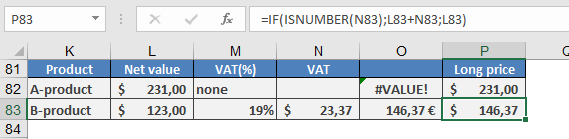
Problem 2: Safe Summation
Error-prone formula:
=L83+N83
Robust solution:
=IF(ISNUMBER(N83); L83+N83; L83)
Pro Tip
Combine with other functions for advanced checks:
=IF(AND(ISNUMBER(A1); A1>0); « Valid »; « Invalid »)
Validates positive numbers only.
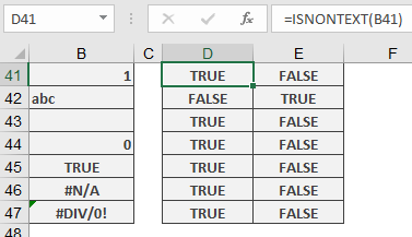
How to use the ISNONTEXT function in Excel
This function returns TRUE if the value is not text (including numbers, errors, logical values, or empty cells). It returns FALSE only if the value is text.
Syntax
ISNONTEXT(value)
Arguments
- value (required): The expression to check (number, text, formula, logical value, error, reference, or name).
Key Features
- Part of the IS() function family – evaluates without type conversion (e.g., « 123 » is treated as text, not a number).
- Returns TRUE for empty cells – unlike some other IS functions.
- Counterpart to ISTEXT():
ISNONTEXT(value) = NOT(ISTEXT(value))
Practical Applications
- Data Validation (Prevent Text Entries)
=ISNONTEXT(B41)
- Use in Data Validation (Custom formula) to block text inputs in a cell while allowing numbers/dates/empty cell
- Location: Data tab → Data Validation → Custom → Enter formula
- Handling Cell Overflow Issues
When long text might spill into adjacent cells:
- Combine with conditional formatting to flag potential display issues
- Use to trigger warnings when formulas generate unexpected text outputs
- Clean Data Processing
=IF(ISNONTEXT(A1), « Numeric Data », « Text Data »)
- Useful for data type categorization in reports
- Helps separate text/non-text entries for different processing
Special Notes:
- Returns TRUE for all error types (#N/A, #VALUE!, etc.)
- Blank cells return TRUE (different from some other IS functions)
- Numeric strings (e.g., « 123 ») are considered TEXT (returns FALSE)
Example Setup:
- Select target cell
- Data → Data Validation → Custom
- Enter: =ISNONTEXT(B41)
- Set error alert style/message
- Copy validation to other cells as needed
This provides robust control over text inputs while allowing all other value types.
How to use the ISNA function in Excel
This function returns TRUE if the value is the #N/A error. Otherwise, it returns FALSE.
Syntax
ISNA(value)
Arguments
- value (required) – The expression to check (a number, text, a formula without an equal sign, a logical value, an error value, a reference, or a name).
Background
- Part of the IS() function family, which evaluates arguments without conversion (e.g., numeric strings remain text).
- Specifically checks for the #N/A error, unlike ISERROR() (which detects all errors) or ISERR() (which excludes #N/A).
- Useful for error handling in lookup functions (VLOOKUP, HLOOKUP, MATCH, etc.).
Example: Handling #N/A in Lookups
Problem:
When using VLOOKUP(), a missing search term returns #N/A, which may disrupt reports or dashboards.
Solution:
Replace #N/A with a custom message while allowing other errors to display normally:
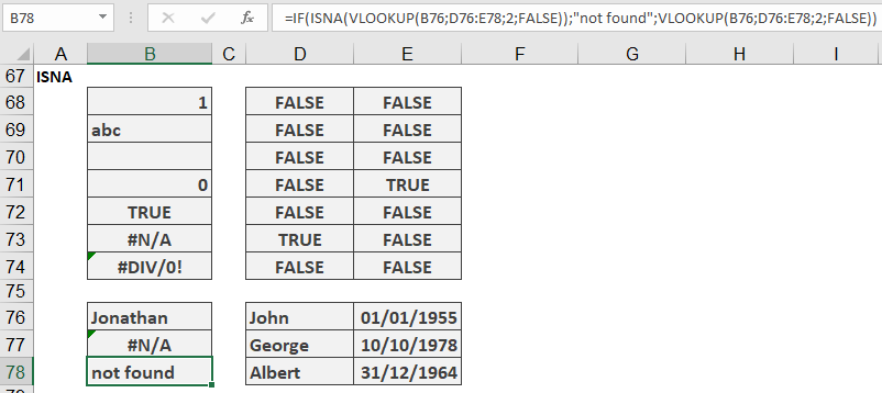
=IF(ISNA(VLOOKUP(B76, D76:E78, 2, FALSE)), « Not found », VLOOKUP(B76, D76:E78, 2, FALSE))
How It Works:
- VLOOKUP(B76, D76:E78, 2, FALSE) searches for B76 in the range D76:D78.
- ISNA() checks if the result is #N/A:
- If TRUE → Returns « Not found ».
- If FALSE → Returns the lookup result (or other errors like #VALUE!).
Key Notes
- Precision: Only suppresses #N/A, preserving other errors (e.g., #REF!, #VALUE!) for debugging.
- Alternatives:
- Use IFERROR() to handle all errors (not just #N/A).
- Combine with IFNA() for cleaner syntax.
When to Use ISNA()
- Data Validation: Flag missing values without masking other errors.
- Conditional Formatting: Highlight cells with #N/A differently from other errors.
How to use the ISLOGICAL function in Excel
This function returns TRUE if the value is a logical value (TRUE or FALSE). Otherwise, it returns FALSE.
Syntax
ISLOGICAL(value)
Arguments
- value (required) – The expression to check (a number, text, a formula without an equal sign, a logical value, an error value, a reference, or a name).
Background
- Part of the IS() function family, which evaluates arguments without conversion (e.g., numeric strings remain text).
- Commonly used with IF() to validate logical conditions before calculations.
- Useful for conditional formatting and data validation rules.
Examples
- Converting Logical Values to Text Messages
Replace TRUE/FALSE with custom messages using nested IF():
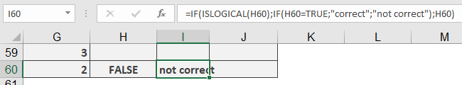
=IF(ISLOGICAL(H60), IF(H60, « Correct », « Not correct »), H60)
- If H60 contains TRUE → Returns « Correct »
- If H60 contains FALSE → Returns « Not correct »
- If H60 is non-logical (e.g., text, number) → Returns the original value.
Key Takeaways
- ISLOGICAL() ensures clean handling of logical values in formulas.
- Combine with IF() for user-friendly outputs or conditional formatting for visual cues.
- Avoids errors by explicitly checking for TRUE/FALSE before processing.