Catégorie : Excel function

The PMT function is used to calculate the total payment required to repay a loan or investment with a fixed interest rate over a specified period. It is particularly useful for determining periodic payments for loans, mortgages, or investments.

The PMT function uses the following syntax for its calculations:

=PMT(rate; nper; pv; [fv]; [type])

• Rate (Required Argument): This is the interest rate for the loan or investment.
• Nper (Required Argument): This represents the total number of payments to be made over the lifetime of the loan or investment.
• Pv (Required Argument): This is the present value, or the total amount that a series of future payments is worth now. It is also referred to as the principal.
• Fv (Optional Argument): This is the future value or the cash balance you aim to achieve after the last payment is made. If omitted, it defaults to 0.
• Type (Optional Argument): This indicates when payments are due. If omitted, it defaults to 0, meaning payments are due at the end of the period. If 1 is used, payments are due at the beginning of the period.

USING THE PMT FUNCTION

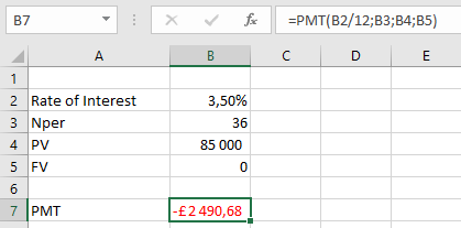
Using the table below, let’s assume we need to invest for three years to receive £85,000 with an annual interest rate of 3,5%. Payments will be made at the start of each month, and the future value is 0.

To calculate the PMT:

1. Select an empty cell and enter the function with its arguments:
   =PMT(B2/12; B3; B4; B5)

1. Press Enter, and the payment amount will be calculated. In this example, the payment is -£2 490,87, as shown in the table below.

IMPORTANT NOTES WHEN USING THE PMT FUNCTION

• A #VALUE! error occurs if non-numeric arguments are provided.
• A #NUM! error occurs if the given interest rate is less than or equal to -1.
• A #NUM! error also occurs if the number of payment periods (nper) is 0.
• When calculating monthly or quarterly payments, ensure the annual interest rate is converted to a monthly or quarterly rate.
• To find the total amount paid over the duration of the loan, multiply the calculated PMT by the total number of payment periods (nper).

The NPV function is used to calculate the net present value of an investment by utilizing a discount rate and a series of future cash flows. It helps determine the profitability of an investment by considering the time value of money.

The NPV function uses the following syntax for its calculations:

=NPV(rate, value1, [value2], …)

• Rate (Required Argument): This is the discount rate applied over the length of a period.
• Value1 (Required Argument): This represents the first value in a series of cash flows, which can include both payments (negative values) and income (positive values). Negative values indicate outgoing payments, while positive values indicate incoming payments.
• Value2 (Optional Argument): This represents additional values in the series of cash flows, following the same rules as Value1.

USING THE NPV FUNCTION

Using the table below, let’s calculate the net present value with the NPV function:

       

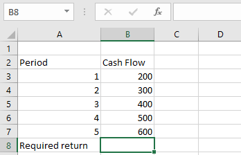
To calculate the net present value;

1. Select an empty cell and enter the function with its arguments:
   =NPV(B9; B3:B8)

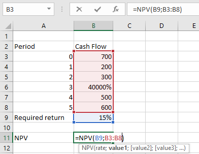
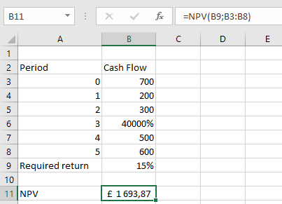
1. Press Enter, and the net present value will be calculated. In this example, the net present value is £1 693,87, as shown in the table below.

IMPORTANT NOTES WHEN USING THE NPV FUNCTION

• All arguments must be numerical or functions that return numerical values. Any other form of input will result in an error.
• In the NPV function, only arrays containing numerical values are evaluated. All other values are ignored.
• The order of cash flow inputs is important and must be entered correctly.
• The NPV function assumes that payments are evenly spaced and occur at regular intervals.
• The NPV function is closely related to the IRR (Internal Rate of Return) function, as both are used to evaluate the profitability of investments.

The FV function is designed to calculate the future value of an investment or loan based on periodic, constant payments and a constant interest rate. It is commonly used to determine the value of an investment or loan at a future point in time.

The FV function uses the following syntax for its calculations:

=FV(rate, nper, pmt, [pv], [type])

• Rate (Required Argument): This is the interest rate per compounding period.
• Nper (Required Argument): This represents the total number of payment periods over the lifetime of the investment or loan.
• Pmt (Optional Argument): This indicates the payment made each period. If this argument is omitted, the pv (present value) argument must be provided.
• Pv (Optional Argument): This represents the present value of the investment or loan. If this argument is omitted, the pmt (payment) argument must be provided.
• Type (Optional Argument): This specifies whether payments are made at the beginning or end of the period. Entering 0 means payments are due at the end of the period, while 1 means payments are due at the beginning.

USING THE FV FUNCTION

Using the information in the table below, let’s calculate the future value with the FV function:            

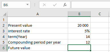
To find the future value of the table above using the FV function

1. Select an empty cell and enter the function with its arguments:
   =FV(B3/B5, B4*B5, 0, -B2)

   

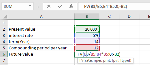
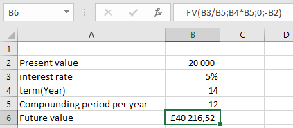
1. Press Enter, and the future value will be calculated. In this example, the future value is £40 216,52, as shown in the table below.

   

IMPORTANT NOTES WHEN USING THE FV FUNCTION

• If non-numeric arguments are provided, the FV function will return a #VALUE! error.
• The payment value (pmt) will appear as a negative number when it represents cash going out of a business (e.g., loan payments or investments).

The PV function, which stands for Present Value, is designed to calculate the present value of an investment or loan based on a constant interest rate. It can be applied to scenarios involving periodic, constant payments, such as mortgages or other loans, or to determine the present value of a future investment goal.

The PV function uses the following syntax for its calculations:

=PV(rate, nper, pmt, [fv], [type])

– Rate (Required Argument): This represents the interest rate per compounding period. For example, a loan with a 14% annual interest rate and monthly payments would have a monthly interest rate of 1.2% (i.e., 14/12 = 1.2%).

– Nper (Required Argument): This is the total number of payment periods required to repay the loan. For instance, a 4-year loan with monthly payments would have 48 payment periods (4 x 12).

– Pmt (Required Argument): This is the fixed payment amount made each period, which remains constant throughout the investment or loan term.

– Fv (Optional Argument): This refers to the future value of the investment at the end of the payment period. If no value is provided, Excel defaults this to 0.

– Type (Optional Argument): This indicates whether payments are made at the beginning or end of the period. Entering 0 means payments are due at the end of the period, while 1 means payments are due at the beginning.

USING THE PV FUNCTION

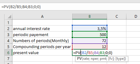
Consider the example of an annuity that makes periodic payments of $500,00 with an annual interest rate of 3,5%. The annuity makes monthly payments over a period of 6 years. To calculate the present value using the PV function, follow these steps:

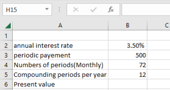
To find the present value of the table above using the PV function

1. Select an empty cell and enter the function with its arguments:

           =PV(B2/B5, B4, B3, 0, 0)

       

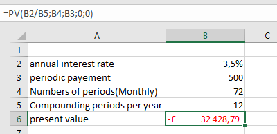
2. Press **Enter**, and the present value will be calculated. In this example, the present value is **-£32 428,79**, as shown in the table below.

       

IMPORTANT NOTES WHEN USING THE PV FUNCTION

– If non-numeric arguments are provided, the PV function will return a `#VALUE!` error.

– The annual interest rate cannot be automatically converted to a periodic rate within the PV function. You must manually convert it before using the function