Votre panier est actuellement vide !
Catégorie : Excel function
How to use the MOD function in Excel
The MOD function returns the remainder after dividing one number (dividend) by another (divisor).
The MOD function uses these arguments:
=MOD(number, divisor)Number (Required): The dividend (number to be divided)
Divisor (Required): The number to divide byUSING THE MOD FUNCTION
Let’s find the remainder of dividing cell A2 by B2 in the table below:
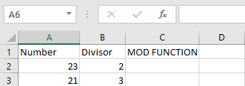
- Select an empty cell
- Enter the formula:
=MOD(A2, B2)- A2 contains the dividend
- B2 contains the divisor
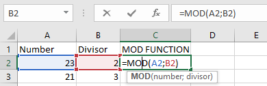
- The result will display in the selected cell
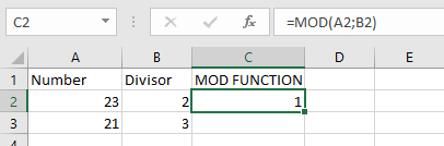
IMPORTANT NOTES
- #DIV/0! error occurs when:
- The divisor is zero
- The result will have:
- The same sign (+/-) as the divisor
How to use the SUMIFS function in Excel
The SUMIFS function adds cells that meet multiple specified conditions. These conditions can evaluate dates, numbers, and text values. The function supports logical operators (<, >, ≤, etc.) and wildcard characters (*, ?).
The SUMIFS function uses these arguments:
=SUMIFS(sum_range, criteria_range1, criteria1, [criteria_range2, criteria2], …)Sum_range: The range of cells to sum
Criteria_range1: The range where the first condition will be applied
Criteria1: The condition that determines which cells to include
Criteria_range2: (Optional) Additional range for second conditionUSING THE SUMIFS FUNCTION

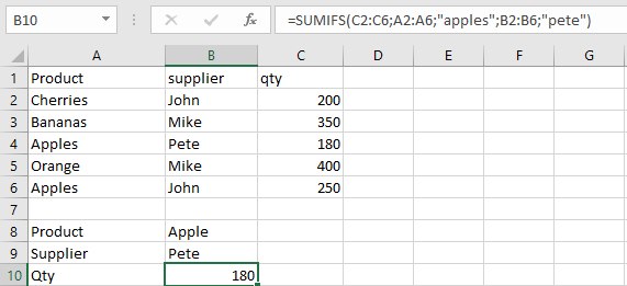
Let’s calculate the total quantity of Apples supplied by Pete:
- Select an empty cell
- Enter the formula:
=SUMIFS(C2:C6, A2:A6, « apples », B2:B6, « Pete »)- C2:C6 contains quantities to sum
- A2:A6 contains product names
- « apples » is our product criteria
- B2:B6 contains supplier names
- « Pete » is our supplier criteria
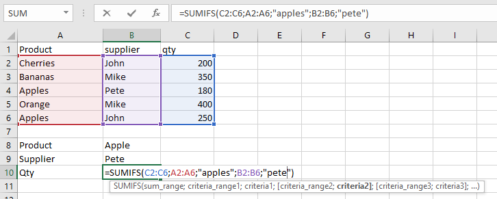
- Press Enter to see the result: 180
IMPORTANT NOTES
- Always enclose text criteria in double quotes (e.g., « orange »)
- All criteria ranges must match the size of sum_range
- #VALUE! error appears when:
- Ranges have different sizes
- Cell references in criteria are incorrectly quoted
- SUMIFS works with cell ranges, not arrays
How to use the SUMIF function in Excel
The SUMIF function calculates the total of cells that meet specific conditions. These conditions can be based on dates, numbers, or text values. The function supports logical operators (<, >, =, etc.) and wildcard characters (*, ?).
The SUMIF function uses these arguments:
=SUMIF(range; criteria; [sum_range])Range (Required):
This is the group of cells that will be checked against your criteria.Criteria (Required):
This determines which cells to include in the sum. You can use:- Numbers (like 10, 0.5, or 12:00)
- Text (such as « January », « North »)
- Expressions (for example, « >100 » or « <=50 »)
Sum_range (Optional):
These are the actual cells to add together. If you leave this out, Excel will sum the cells in your range instead.HOW TO USE SUMIF FUNCTION
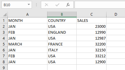
Let’s see how this works with two practical examples: calculating January sales using the table below;
Example 1: Calculate January Sales
- Click on an empty cell
- Type the formula:
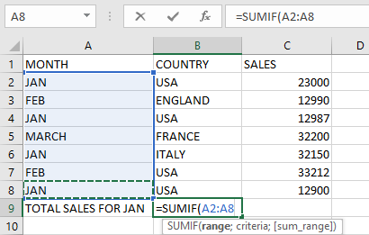
=SUMIF(A2:A8; « Jan »; C2:C8)- A2:A8 contains month names
-
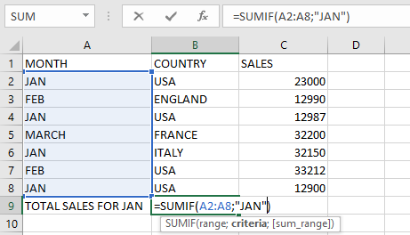
- « Jan » is our condition
-
- C2:C8 has the sales numbers
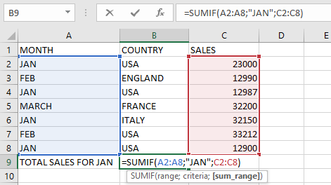
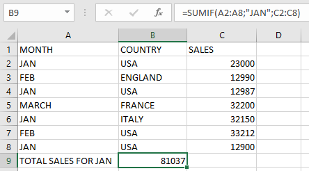
- Press Enter to see the result: 81037
Example 2: Calculate USA Sales
- Select an empty cell
- Enter the formula:
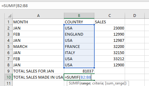
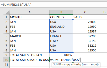
=SUMIF(B2:B8; « USA »; C2:C8)- B2:B8 lists countries
-
- « USA » is our criteria
-
- C2:C8 contains the sales figures
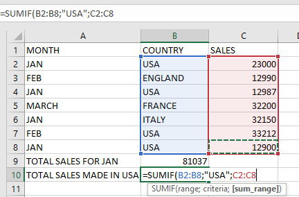
- Hit Enter to view the total USA sales
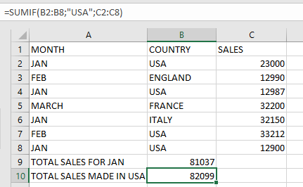
IMPORTANT NOTES
- If you see #VALUE!, your criteria might be too long (over 255 characters)
- When you don’t specify sum_range, Excel sums the cells in your range
- Always put text criteria in « double quotes »
- Wildcards work in SUMIF:
- matches multiple characters (e.g., « A* » finds « Apple »)
-
- ? matches one character (e.g., « J?n » finds « Jan » or « Jun »)
How to use the SUM function in Excel
The SUM function adds or totals the values of selected cells, rows, or columns.
Syntax
=SUM(number1, [number2], …)
How to Insert the SUM Function
- Select a cell and type =SUM(.
- In the function arguments, select the desired cells or range.
- Press Enter to display the result.
Arguments
- number1 (Required): The first value or range to sum.
- [number2], [number3], … (Optional): Additional values or ranges to include in the sum.
USING THE SUM FUNCTION
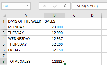
Example: Calculate the total sales from Monday to Friday.
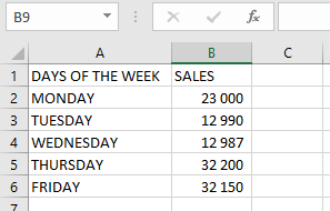
To calculate the sales from Monday to Friday using SUM, follow the steps below
Steps:
- Select an empty cell.
- Enter the function with the cell range:
=SUM(A2:B6)
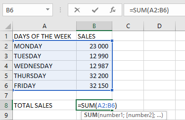
- Press Enter—the result (e.g., 113,327) will appear.
NOTES WHEN USING THE SUM FUNCTION
- #VALUE! Error: Occurs if the criteria exceed 255 characters.
- Ignored Cells: The SUM function automatically skips empty cells and text values.
- Valid Arguments: Can include constants, ranges, named ranges, or cell references.
- Error Handling: If any argument contains an error, the SUM function returns an error.
How to use the FIND function in Excel
Similar to the SEARCH function, the FIND function also locates the position of a substring within a string. However, unlike the SEARCH function, the FIND function is case-sensitive, meaning it distinguishes between uppercase and lowercase letters when searching for the exact text.
The syntax for the FIND function is:
=FIND(find_text; within_text; [start_num])- find_text: The text or substring you want to find.
- within_text: The text in which you want to search for the substring.
- start_num (optional): The position in the text where the search should begin. If omitted, the search starts from the first character.
Practical Example of the FIND Function
Example 1:
Find the position of « GROWTH » in cell B2 in the table below.
- Go to cell C2 and type:
=FIND(« GROWTH »; B2; 1) - Press Enter.

The position of « GROWTH » in cell B2 is 22.
How to use the SEARCH function in Excel
The SEARCH function is used to locate the position of a substring within a string. For example, it can find the position of the letter « S » in the word « JOURNALISM. » The SEARCH function is case-insensitive, meaning it does not distinguish between uppercase and lowercase letters.
The syntax for the SEARCH function is:
=SEARCH(find_text; within_text; [start_num])- find_text: The text or substring you want to find.
- within_text: The text in which you want to search for the substring.
- start_num (optional): The position in the text where the search should begin. If omitted, the search starts from the first character.
Practical Examples of the SEARCH Function
Example 1:
Search for the position of « T » in cell A1 in the table below.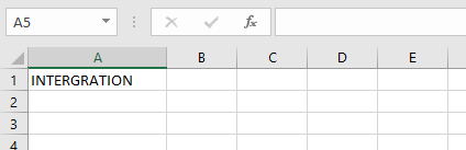
- Go to cell B2 and type:
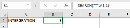
=SEARCH(« T »; A1; 1)
- Press Enter.
The position of « T » in cell A1 is 3.
Example 2:
Search for the position of « MAN » in cell C1 in the table below.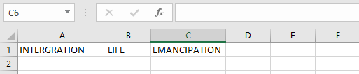
- Go to cell D2 and type:
=SEARCH(« MAN »; C1; 1)S
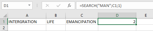
- Press Enter.
The position of « MAN » in cell D1 is 2.
How to use the DDB function in Excel
The DDB function calculates the depreciation of an asset for a specific period using the double-declining balance method or another specified method by adjusting the factor argument. It uses the following arguments:
=DDB(cost; salvage; life; period; [factor])
- Cost (Required Argument): This is the initial cost of the asset.
- Salvage (Required Argument): This is the value of the asset at the end of its depreciation, also known as the salvage value.
- Life (Required Argument): This is the number of periods over which the asset depreciates, often referred to as the asset’s useful life.
- Period (Required Argument): This is the specific period for which the depreciation is calculated.
- Factor (Optional Argument): This is the rate at which the balance declines. If omitted, it defaults to 2 (double-declining balance method).
Using the DDB Function
Let’s calculate the depreciation of an asset with an initial cost of £300 000, a salvage value of £5 000 after 5 years, and a depreciation period of 2 years. We will use the DDB function with a factor of 1.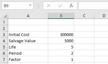
To calculate the depreciation using the DDB function:
- Select an empty cell and enter the function with its arguments:
=DDB(B3; B4; B5; B6; B7)
(Where B3 = Cost, B4 = Salvage, B5 = Life, B6 = Period, B7 = Factor)
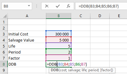
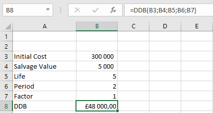
- Press Enter, and the depreciation value of the asset will be displayed as £48000,00, as shown in the table below.
Important Notes When Using the DDB Function
- A #VALUE! error occurs if any of the arguments provided are non-numeric.
- A #NUM! error occurs in the following cases:
- If the cost or salvage value is less than 0.
- If the life of the asset is less than or equal to zero.
- If the period argument is less than or equal to 0 or greater than the life value.
- If the factor argument is less than 1.
How to use the DB function in Excel
The DB function calculates the depreciation of an asset using the fixed declining balance method for a specified period. It utilizes the following arguments to perform its operations:
=DB(cost; salvage; life; period; [month])
- Cost (Required Argument): This is the initial cost of the asset.
- Salvage (Required Argument): This is the value of the asset at the end of its depreciation, also known as the salvage value.
- Life (Required Argument): This represents the number of periods over which the asset depreciates, often referred to as the asset’s useful life.
- Period (Required Argument): This is the specific period for which the depreciation is calculated.
- Month (Optional Argument): This indicates the number of months in the first year used for depreciation calculation. If omitted, the function defaults to 12 months.
Using the DB Function
Let’s calculate the depreciation of an asset with an initial cost of £200 000, a salvage value of £8 000 after 5 years, and a depreciation period of 2 years with 4 months in the first year.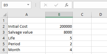
To find the depreciation value using the DB function:
- Select an empty cell and enter the function with its arguments:
=DB(B2; B3; B4; B5; B6)
(Where B2 = Cost, B3 = Salvage, B4 = Life, B5 = Period, B6 = Month)
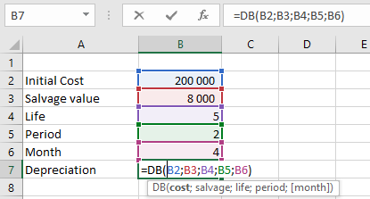
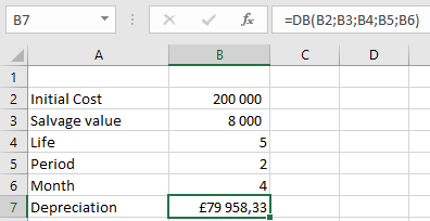
- Press Enter, and the depreciation value of the asset will be displayed as £79958,33, as shown in the table below.
Important Notes When Using the DB Function
- A #VALUE! error occurs if any of the arguments provided are non-numeric.
- A #NUM! error occurs in the following cases:
- If the cost or salvage value is less than zero.
- If the life or period argument is less than or equal to zero.
- If the month argument is less than or equal to zero or greater than 12.
- If the period argument is greater than the life argument and the month argument is omitted.
- If the period provided is greater than life + 1.
How to use the SYD FUNCTION in Excel
The SYD function is used to calculate the sum-of-years’ depreciation of an asset over a specific period within its useful life. This method focuses on the initial cost of the asset, its salvage value, and the number of periods over which the asset depreciates.
The SYD function uses the following syntax for its calculations:
=SYD(cost; salvage; life; per)
- Cost (Required Argument): This is the initial cost of the asset.
- Salvage (Required Argument): This is the value of the asset at the end of its useful life, also known as the salvage value.
- Life (Required Argument): This represents the total number of periods over which the asset depreciates, often referred to as the useful life of the asset.
- Per (Required Argument): This is the specific period for which the depreciation is being calculated.
USING THE SYD FUNCTION
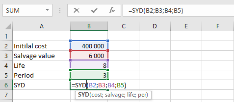
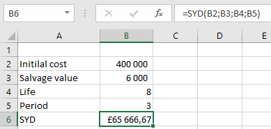
Let’s assume we want to calculate the depreciation of an asset with an initial cost of £400 000, a salvage value of £6 000, and a useful life of 8 years. We want to calculate the depreciation for the 3rd year.
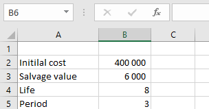
To calculate the sum-of-years’ depreciation:
- Select an empty cell and enter the function with its arguments:
=SYD(B2; B3; B4, B5)
- Press Enter, and the depreciation value for the specified period will be calculated. In this example, the depreciation value is £65 666,67, as shown in the table below.
IMPORTANT NOTES WHEN USING THE SYD FUNCTION
- The life and per arguments must use the same units of time (e.g., days, months, or years).
- A #VALUE! error occurs if any of the arguments provided are non-numeric.
- A #NUM! error occurs in the following cases:
- If the salvage value is less than zero.
- If the life or per argument is less than or equal to zero.
- If the per argument is greater than the life argument.
How to use the SLN function in Excel
The SLN function is used to calculate the depreciation of an asset using the straight-line depreciation method for a single period. This method evenly spreads the cost of the asset over its useful life.
The SLN function uses the following syntax for its calculations:
=SLN(cost; salvage; life)
- Cost (Required Argument): This is the initial cost of the asset.
- Salvage (Required Argument): This is the value of the asset at the end of its useful life, also known as the salvage value.
- Life (Required Argument): This represents the number of periods over which the asset depreciates, often referred to as the useful life of the asset.
USING THE SLN FUNCTION
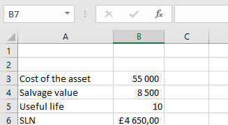
Using the table below, let’s calculate the depreciation of an asset with an initial cost of £55000, a salvage value of £8 500, and a useful life of 10 years.
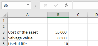
To calculate the depreciation:
- Select an empty cell and enter the function with its arguments:
=SLN(B3; B4; B5)
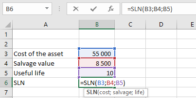
- Press Enter, and the depreciation value will be calculated. In this example, the depreciation value is £4 650,00, as shown in the table below.
IMPORTANT NOTES WHEN USING THE SLN FUNCTION
- A #DIV/0! error occurs if the life argument is equal to zero.
- A #VALUE! error occurs if any of the arguments provided are non-numeric.