Votre panier est actuellement vide !
Catégorie : Excel function
How to use the AVERAGE function in Excel
The AVERAGE function calculates the arithmetic mean of a specified set of values in a worksheet. This function can accept up to 255 arguments, including cell references, ranges, arrays, and constants.
The AVERAGE function uses the following arguments:
=AVERAGE(number1; [number2]; …)
Number1 (Required Argument): The first number, cell reference, or range for which you want to calculate the average.
Number2 (Optional Argument): Additional numbers, cell references, or ranges to include in the average calculation (up to 255 total arguments).USING THE AVERAGE FUNCTION
Let’s calculate the average sales of goods in the table below using the AVERAGE function.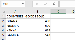
To find the average sales:
- Select an empty cell and enter:
=AVERAGE(B2:B5)
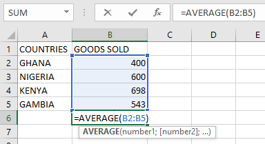
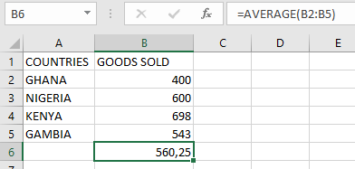
- Press Enter to display the result: 560,25 (as shown in the table below).
NOTE: Important considerations when using the AVERAGE function:
- Empty cells are automatically excluded from the calculation
- Text and logical values in cell references are ignored
- Cells containing zero (0) are included in the calculation
- All referenced cells must contain numeric values
- To include logical values and text representations of numbers, use the AVERAGEA function
- For conditional average calculations, use the AVERAGEIF or AVERAGEIFS functions
How to use the COUNTBLANK function in Excel
The COUNTBLANK function calculates the number of empty cells within a specified range in a worksheet.
The COUNTBLANK function requires a single argument:
=COUNTBLANK(range)
Range (Required Argument): This specifies the cell range where blank cells should be counted.
USING THE COUNTBLANK FUNCTION
Let’s determine the number of blank cells in the table below using the COUNTBLANK function.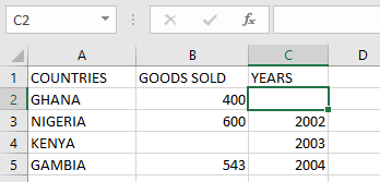
To count blank cells, follow these steps:
- Select an empty cell and enter:
=COUNTBLANK(A1:C5)
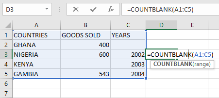
- Press Enter to display the result: 2 (as shown in the table below).
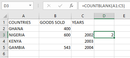
NOTE: Important notes when using the COUNTBLANK function:
- Excludes cells containing text, numbers, errors, or other non-blank values
- Counts cells with formulas that return empty results as blank
- Does not count cells containing zeros (0) as blank
How to use the COUNTA function in Excel
The COUNTA function is a function that returns the number of non-empty cells within a specified range. This function excludes empty cells from its count. The COUNTA function may also be known as the Excel COUNTIF Not Blank formula.
The COUNTA function uses the following arguments:
=COUNTA(value1; [value2]; …)
Value1 (Required Argument): This represents the first set of values to be counted.
Value2,… (Optional Argument): These are additional values to include in the count, with a maximum of 255 total arguments permitted.USING THE COUNTA FUNCTION
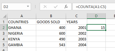
Using the table below, we will determine the number of non-empty cells by applying the COUNTA function.
To calculate the quantity of non-empty cells in your worksheet, follow these steps:
- Select an empty cell and input:
=COUNTA(A1:C5)

- Press Enter to display the result: 15 (as illustrated in the table below).
NOTE: Important considerations when working with the COUNTA function:
- Empty cells are automatically excluded from the count
- For counts excluding logical values, text, or error messages, utilize the COUNT function instead
- To implement conditional counting based on specific criteria, employ either the COUNTIF or COUNTIFS functions
How to use the COUNTIFS function in Excel
The COUNTIFS function is a function used for counting cells that meet single or multiple conditions or criteria. Just like the COUNT and COUNTIF functions, the COUNTIFS function is used with criteria or conditions relating to numbers, dates, text, logical operators, and wildcards.
The COUNTIFS function has the following arguments:
=COUNTIFS(criteria_range1; criteria1; [criteria_range2; criteria2]…)
Criteria_range1 (Required Argument): This is the first range to be evaluated with the associated criteria.
Criteria1 (Required Argument): This is the condition to be applied to criteria_range1, which may be an expression, number, cell reference, or text specifying which cells to count. For example, criteria can be expressed as 43, « >23 », D2, etc.
Criteria_range2, criteria2 (Optional Argument): These are additional ranges and their associated criteria. The function allows up to 127 range/criteria pairs. The criteria can be:- A numerical value (integer, decimal, time, or logical value)
- A text string (e.g., « Monday », « East », « Price ») including wildcards (*, ?)
USING THE COUNTIFS FUNCTION
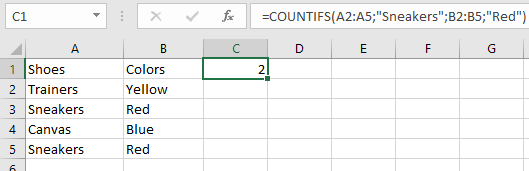
Using the table below, let’s count the number of shoes that are red.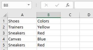
To count red shoes in the list, follow these steps:
- Select an empty cell and enter:
=COUNTIFS(A2:A5; « sneakers »; B2:B5; « red »)
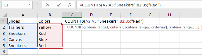
- Press Enter. The result will be 2, as shown in the table.
NOTE: Remember these points when using COUNTIFS:
- COUNTIFS treats empty cells as 0 when criteria reference an empty cell.
- #VALUE! error occurs if:
- Criteria ranges have different lengths
- Text criteria exceed 255 characters
- Wildcards (*, ?) can be used in criteria.
- The function evaluates each cell pair sequentially:
- If the first cell pair meets criteria, count increases by 1
- If the second pair meets criteria, count increases again by 1
- This continues until all cells are evaluated
How to use the COUNTIF function in Excel
The COUNTIF function is used to count the number of cells that meet a certain criterion or condition. This can also be used to count cells that contain dates, numbers, and text. This function also supports the use of logical operators and wildcards.
The COUNTIF function has the following arguments:
=COUNTIF(Range; criteria)
Range (Required Argument): This indicates the range of cells that are to be counted.
Criteria (Required Argument): This is the condition to be met by the cells provided in the worksheet. The criteria can be in the following:- A numerical value such as integer, decimal, time, or logical value
- A text string such as Monday, East, Price and including wildcards such as asterisks and question mark
USING THE COUNTIF FUNCTION
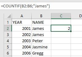
With the table below, let’s use the COUNTIF function to count how many times James’ name appears on the list.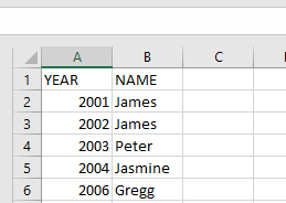
To get the number of times James’ name appears on the list, follow the steps below:
- Select an empty cell, type in the function name and the arguments to be used:
=COUNTIF(B2:B6; « James »)
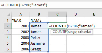
- Click on Enter and the result will be 2.
NOTE: Take note of the following points when using the COUNTIF function:
- When using the COUNTIF function, make sure the criteria argument is enclosed in quotes (e.g., « James »).
- When the provided criteria argument is a text string that is more than 255 characters in length, #VALUE! error occurs.
- #VALUE! error also occurs when the formula is referring to a cell or range of cells in a closed workbook.
How to use the COUNT function in Excel
The COUNT function is a function that counts the number of cells containing numbers, as well as the number of arguments that include numerical values.
The COUNT function uses the following syntax:
- Value1 (Required Argument): The cell range or value you want to include in the count (must contain numbers).
- Value2, … (Optional Argument): You can add up to 255 additional items, cell references, or ranges where numbers should be counted.
USING THE COUNT FUNCTION
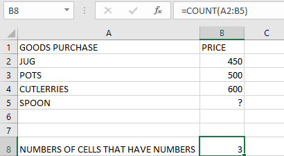
Using the table below, we will count how many cells contain numbers with the COUNT function.
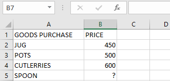
To count cells with numbers, follow these steps:
- Select an empty cell.
- Type the function followed by the range:
=COUNT(A2:B5)

Press Enter. The result will be 3.
NOTE: IMPORTANT POINTS ABOUT THE COUNT FUNCTION
- Counted Values: Numbers, dates, and text representations of numbers (e.g., « 10 »).
- Not Counted: Text values, errors, or empty cells.
- For counting logical values (TRUE/FALSE), use COUNTA.
- For counting numbers based on conditions, use COUNTIF or COUNTIFS.
- The COUNT function does not count logical values (TRUE or FALSE).
- If an argument is an array or reference, only numbers within it are counted.
How to use the ROUNDUP function in Excel
The ROUNDUP function rounds a number up (away from zero) to a specified number of digits.
The ROUNDUP function uses these arguments:
=ROUNDUP(number, num_digits)Number (Required): The value you want to round up
Num_digits (Required): The number of digits to round toUSING THE ROUNDUP FUNCTION
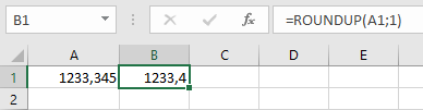
Let’s round up 1233,345 to various precision levels:
- One decimal place:
=ROUNDUP(A1; 1) → Returns 1233,4
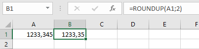
- Two decimal places:
=ROUNDUP(A1; 2) → Returns 1233,35
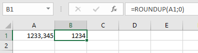
- Nearest integer:
=ROUNDUP(A1; 0) → Returns 1234
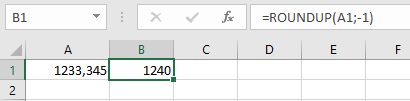
- Nearest 10:
=ROUNDUP(A1; -1) → Returns 1240
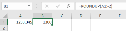
- Nearest 100:
=ROUNDUP(A1; -2) → Returns 1300
- Nearest 1000:
=ROUNDUP(A1; -3) → Returns 2000
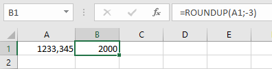
Note: Unlike the standard ROUND function, ROUNDUP always rounds numbers upward regardless of the digit value.
- One decimal place:
How to use the ROUND function in Excel
The ROUND function adjusts a number to a specified number of digits, either rounding up or down as needed.
The ROUND function uses these arguments:
=ROUND(number, num_digits)Number (Required): The value you want to round
Num_digits (Required): The number of decimal places to round toUSING THE ROUND FUNCTION
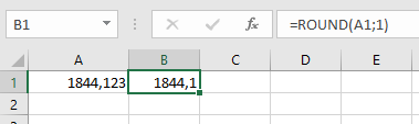
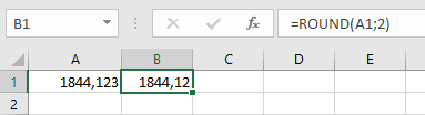
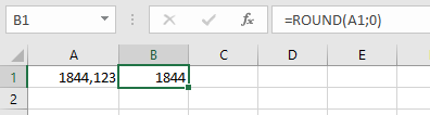
Let’s round the number 1844,123 to various precision levels:
- One decimal place:
=ROUND(A1; 1)→ Returns 1844,1
- Two decimal places:
=ROUND(A1; 2)→ Returns 1844,12
- Nearest integer:
=ROUND(A1; 0)→ Returns 1844
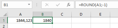
- Nearest 10:
=ROUND(A1; -1)→ Returns 1840
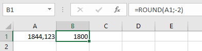
- Nearest 100:
=ROUND(A1; -2)→ Returns 1800
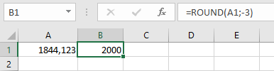
- Nearest 1000:
=ROUND(A1; -3)→ Returns 2000
Note: Positive num_digits rounds decimal places, zero rounds to whole numbers, and negative num_digits rounds to left of the decimal point.
- One decimal place:
How to use the ROUNDDOWN function in Excel
The ROUNDDOWN function rounds a number down (toward zero) to a specified number of digits.
The ROUNDDOWN function uses these arguments:
=ROUNDDOWN(number; num_digits)Number (Required): The value you want to round down
Num_digits (Required): The number of digits to round toUSING THE ROUNDDOWN FUNCTION
Let’s round down 1233,345 to various precision levels:
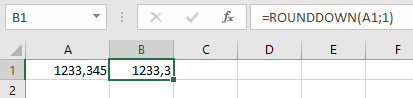
- One decimal place:
=ROUNDDOWN(A1; 1) → Returns 1233,3
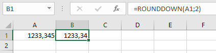
- Two decimal places:
=ROUNDDOWN(A1; 2) → Returns 1233,34
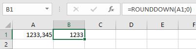
- Nearest integer:
=ROUNDDOWN(A1; 0) → Returns 1233
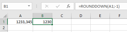
- Nearest 10:
=ROUNDDOWN(A1; -1) → Returns 1230
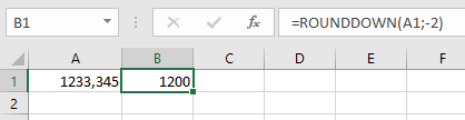
- Nearest 100:
=ROUNDDOWN(A1; -2) → Returns 1200
- Nearest 1000:
=ROUNDDOWN(A1; -3) → Returns 1000
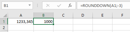
Note: Unlike the standard ROUND function, ROUNDDOWN always rounds numbers downward regardless of the digit value.
- One decimal place:
How to use the RANDBETWEEN function in Excel
The RANDBETWEEN function generates a random integer between two specified numbers. This function recalculates automatically whenever the worksheet is opened or modified.
The RANDBETWEEN function uses these arguments:
=RANDBETWEEN(bottom, top)Bottom (Required): The smallest integer that can be returned
Top (Required): The largest integer that can be returnedUSING THE RANDBETWEEN FUNCTION
To see how this function works, examine the following example:
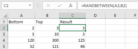
- The formula =RANDBETWEEN(A2; B2) has been applied above
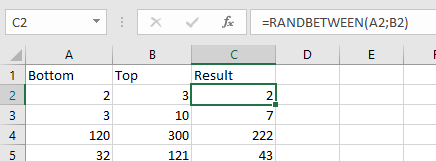
- Each time the worksheet recalculates, a new random number appears as seen below;
IMPORTANT NOTES
- The function generates a new value with each worksheet recalculation
- To prevent automatic recalculation:
- Enter the formula in the formula bar
- Press F9 to convert it to a static value
- To generate multiple random numbers at once:
- Select multiple cells
- Enter the RANDBETWEEN function
- Press Ctrl + Enter to fill all selected cells