Votre panier est actuellement vide !
Étiquette : excel_vba
How to Calculate the Average in Excel
In mathematics, the average (more precisely the arithmetic mean) is calculated by summing a group of numbers and then dividing that total by the count of the numbers.
For example, if three athletes complete a race in 10.5 seconds, 10.7 seconds, and 11.2 seconds respectively, the average time would be:
= (10.5 + 10.7 + 11.2) / 3,
which gives 10.8 seconds.However, in Excel, you don’t need to write this kind of mathematical expression manually. Excel provides powerful built-in functions such as AVERAGE() that automatically handle these calculations.
AVERAGE() Function
The AVERAGE() function in Excel returns the arithmetic mean of the specified numbers. Its syntax is:
=AVERAGE(number1, [number2], …)
- number1, number2, etc., are the values you want to average. The first argument is required, and up to 255 arguments are allowed.
- These values can be numbers, cell references, or ranges.
How to Use AVERAGE()
The AVERAGE() function is one of the simplest and most frequently used in Excel. Here are some practical examples:
- To calculate the average of numbers directly:
=AVERAGE(1, 2, 3, 4) → returns 2.5 - To average an entire column:
=AVERAGE(A:A) - To average an entire row:
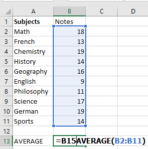
=AVERAGE(1:1) - To average a specific range:
=AVERAGE(B2:B11)
Without the AVERAGE function, you’d have to manually input:
=(B2+B3+B4+…+B11)/10,
or use:
=SUM(B2:B11)/COUNT(B2:B11)You can also average non-contiguous cells:
=AVERAGE(A1, C1, D1)Mixed input types (ranges, values, references) are supported:
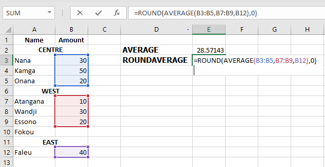
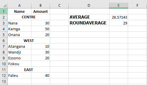
=AVERAGE(B3:B5, B7:B9, B12)To round the result to the nearest whole number:
=ROUND(AVERAGE(B3:B5, B7:B9, B12), 0)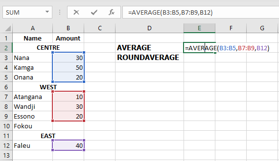
You can also average percentages or times.
Important: The AVERAGE() function includes zero values. If you want to ignore zeros, use AVERAGEIF() instead.
AVERAGE() – Key Notes
- Zeros are included in the average.
- Empty cells, text, Boolean values (TRUE, FALSE) are ignored—unless typed directly in the formula, in which case TRUE=1, FALSE=0.
- Distinguish between zero and an empty cell: zeros are counted, blanks are not. This is affected by the « Show a zero in cells that have zero value » Excel setting (File > Options > Advanced).
AVERAGEA() Function
AVERAGEA() works like AVERAGE() but includes all non-empty cells, including:
- Numbers
- Text (treated as 0)
- Logical values (TRUE = 1, FALSE = 0)
=AVERAGEA(value1, [value2], …)
Examples:
- =AVERAGEA(2, FALSE) → returns 1
- =AVERAGEA(2, TRUE) → returns 1.5
AVERAGEIF() Function
AVERAGEIF() calculates the average of cells that meet a specific condition.
Syntax:
=AVERAGEIF(range, criteria, [average_range])
Where:
- range: cells to test
- criteria: the condition
- average_range (optional): cells to average if different from range
Examples:
Exact match:
=AVERAGEIF(A2:A9, « Orange », B2:B9)
Or using a cell reference:
=AVERAGEIF(A2:A9, E1, B2:B9)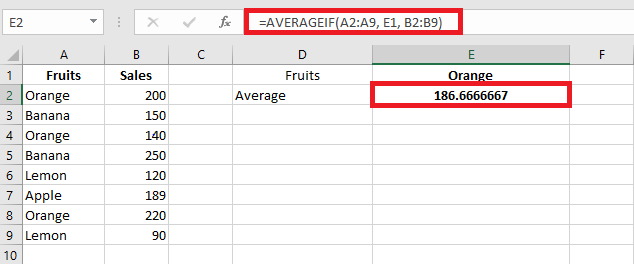
Rounded result:
=ROUND(AVERAGEIF(A2:A9, « Orange », B2:B9), 2)Partial match (wildcards):
- * for any sequence
- ? for a single character
E.g., average all « Orange »-related items:
=AVERAGEIF(A2:A9, « Orange* », B2:B9)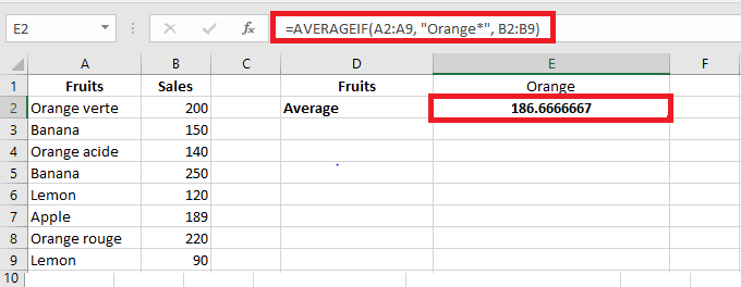
Exclude « Orange »:
=AVERAGEIF(A2:A9, « <>*Orange* », B2:B9)Numeric conditions:
Average values greater than 20:
=AVERAGEIF(A2:A10, « >20 »)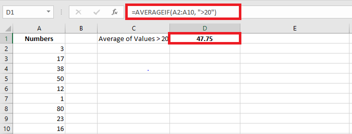
Exclude zeros:
=AVERAGEIF(A2:A10, « <>0 »)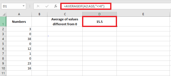
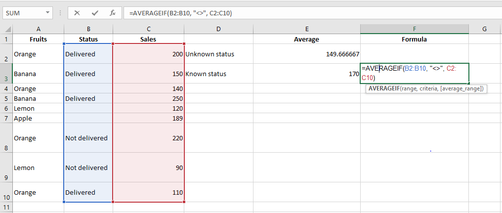
Empty/non-empty cells:
- Empty: =AVERAGEIF(B2:B10, « = », C2:C10)
- Textually blank (e.g. = » »): =AVERAGEIF(B2:B10, « », C2:C10)
- Non-empty: =AVERAGEIF(B2:B10, « <> », C2:C10)
AVERAGEIFS() Function
AVERAGEIFS() averages cells that meet multiple conditions (AND logic).
Syntax:
=AVERAGEIFS(average_range, criteria_range1, criteria1, [criteria_range2, criteria2], …)
Examples:
Multiple conditions:
Average sales of « Orange » where sales > 100:
=AVERAGEIFS(B2:B10, A2:A10, « Orange », B2:B10, « >100 »)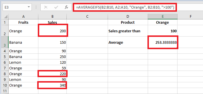
Date conditions:
Average quantity delivered before 21-Aug-2022 with a non-empty status:
=AVERAGEIFS(D2:D10, B2:B10, « <21/08/2022 », C2:C10, « <> »)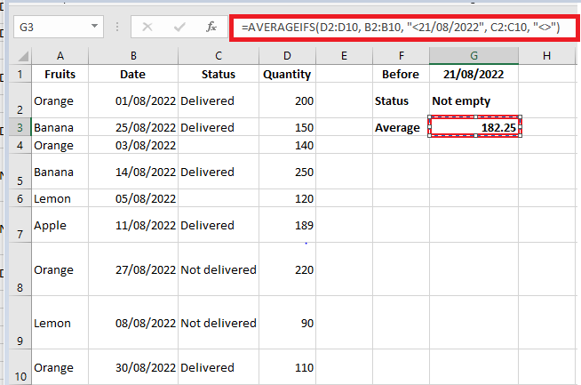
Important Notes on AVERAGEIF and AVERAGEIFS
- Empty or non-numeric cells in average_range are ignored.
- If no cells match criteria, the result is #DIV/0!.
- In AVERAGEIF(), the average_range doesn’t need to match the size of the range, but the top-left cell determines alignment.
- In AVERAGEIFS(), all criteria ranges must match the size of average_range.
How to Average with OR Logic (Multiple Conditions)
Since AVERAGEIFS() uses AND logic, to apply OR logic, you’ll need custom formulas.
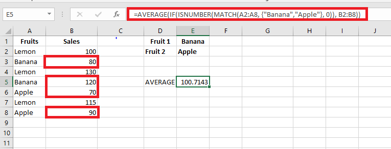
Example 1: OR logic with text values
Average sales of « Banana » or « Apple »:
=AVERAGE(IF(ISNUMBER(MATCH(A2:A8, {« Banana », « Apple »}, 0)), B2:B8))
Or using cell references (e.g. E1:E2 contain « Banana » and « Apple »):
=AVERAGE(IF(ISNUMBER(MATCH(A2:A8, E1:E2, 0)), B2:B8))
Press Ctrl + Shift + Enter to confirm (array formula).
Example 2: OR logic with numeric conditions
Average sales in column D where either column C or D > 50:
=SUM(IF(((C2:C8>50)+(D2:D8>50))>0, D2:D8, 0)) / SUM(–((C2:C8>50)+(D2:D8>50)>0))
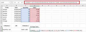
Adaptable for different thresholds, e.g. D2:D8>100.
Example 3: OR logic with empty/non-empty cells
Non-empty cells in column B or C:
=SUM(IF(((B2:B8<> » »)+(C2:C8<> » »))>0, D2:D8, 0)) / SUM(–(((B2:B8<> » »)+(C2:C8<> » »))>0))
Empty cells in column B or C:
=SUM(IF(((B2:B8= » »)+(C2:C8= » »))>0, D2:D8, 0)) / SUM(–(((B2:B8= » »)+(C2:C8= » »))>0))
Conclusion
Excel offers powerful and flexible ways to calculate averages using functions like AVERAGE(), AVERAGEA(), AVERAGEIF(), and AVERAGEIFS(). You can also craft custom formulas to implement OR logic or handle special cases such as blank cells and conditional criteria. With the right understanding, you can efficiently analyze your data in virtually any scenario.
Weighted Average Calculation in Excel
Although Microsoft Excel does not provide a specific weighted average function, it has several other functions that can be used to perform this calculation, as shown in the examples below.
What is a Weighted Average?
A weighted average is a type of arithmetic average where some elements in the data set carry more importance than others. In other words, each value being averaged is assigned a certain weight.
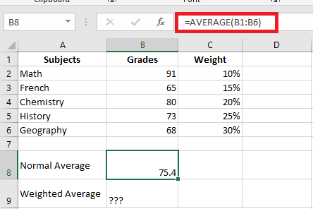
Student grades are often calculated using a weighted average. For example, a regular average is easily calculated using Excel’s AVERAGE() function. However, when we need the average to account for the weight of each activity listed in column C, a weighted average formula is necessary.
In mathematics and statistics, the weighted average is calculated by multiplying each value in the set by its respective weight, then adding these products together and dividing the sum of the products by the sum of all the weights.
For instance, to calculate the weighted average (overall grade), you multiply each score by its corresponding percentage (converted to decimal form), sum the 5 products, and then divide by the sum of the 5 weights:
((91*0.1)+(65*0.15)+(80*0.2)+(73*0.25)+(68*0.3)) / (0.1+0.15+0.2+0.25+0.3) = 73.5
As you can see, the regular average (75.4) and the weighted average (73.5) are different values.
Calculating the Weighted Average
In Microsoft Excel, you can calculate the weighted average using the same approach but with much less effort, as Excel’s functions will do most of the work for you.
Example 1: Calculating the Weighted Average Using the SUM() Function
If you are familiar with the basic SUM() function in Excel, the formula below will require little explanation:
=SUM(B2*C2, B3*C3, B4*C4, B5*C5, B6*C6) / SUM(C2:C6)
Essentially, it performs the same calculation as described above, but using cell references instead of numbers.
As shown in the screenshot, the formula returns exactly the same result as the previous manual calculation. Notice the difference between the regular average (calculated using AVERAGE() in C8) and the weighted average (calculated in C9).
Although the SUM() formula is simple and easy to understand, it’s not the best choice if you have a large number of elements to average. In this case, you should use the SUMPRODUCT() function as shown in the next example.
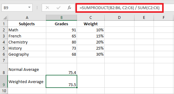
Example 2: Finding a Weighted Average with the SUMPRODUCT() Function
Excel’s SUMPRODUCT() function is perfect for this task as it is designed to sum products, which is exactly what we need. Instead of multiplying each value by its weight individually, you provide two arrays in the SUMPRODUCT() formula (in this context, an array is a continuous range of cells), then divide the result by the sum of the weights:
=SUMPRODUCT(values_range, weights_range) / SUM(weights_range)
Assuming the values to be averaged are in cells B2:B6 and the weights are in cells C2:C6, our SUMPRODUCT() formula for the weighted average looks like this:
=SUMPRODUCT(B2:B6, C2:C6) / SUM(C2:C6)
To view the actual values behind an array, select it in the formula bar and press the F9 key. The result will look something like this:
=SUMPRODUCT(91*0.1 + 65*0.15 + 80*0.2 + 73*0.25 + 68*0.3)
What the SUMPRODUCT() function does is multiply the 1st value in array1 by the 1st value in array2 (910.1 in this example), then multiply the 2nd value in array1 by the 2nd value in array2 (650.15), and so on. After all multiplications are done, the function adds the products and returns that sum.
To ensure the SUMPRODUCT() function gives the correct result, you can compare it to the SUM() formula from the previous example, and you’ll find the numbers are identical.
Excel’s SUM() or SUMPRODUCT() for Weighted Averages
- The weights don’t necessarily need to add up to 100%, and they don’t have to be expressed as percentages.
- For example, you can create a priority scale and assign a certain number of points to each item, just like in the example above.
With these formulas, you can easily calculate a weighted average in Excel without manually multiplying and adding each value. Excel’s functions will handle most of the heavy lifting for you.
Buttons: « Cancel », « Retry », and « Ignore » in Excel VBA
An example featuring three buttons: CANCEL, RETRY, and IGNORE, accompanied by a warning icon. The associated VBA code is as follows:
Sub MsgBoxAbortRetryIgnore()
    Dim response As Integer
    response = MsgBox("An error occurred during the save process." _
        & vbCrLf & "Do you want to cancel the operation?" _
        & vbCrLf & "Do you want to retry the operation?" _
        & vbCrLf & "Do you want to ignore this message?", _
        vbAbortRetryIgnore Or vbExclamation, _
        "Save Error")
    If response = vbAbort Then
        MsgBox "You chose to cancel the operation."
    ElseIf response = vbRetry Then
        MsgBox "You chose to retry the operation."
    Else
        MsgBox "You chose to ignore the message."
    End If
End Sub
Explanation:
This example demonstrates how to create a message box with three distinct buttons — Cancel, Retry, and Ignore — that allows the user to respond to a critical situation such as an error during a save process. These buttons provide the user with options to either cancel the operation, retry it, or ignore the warning altogether.
The message box also includes a warning symbol (the exclamation mark icon) to clearly indicate the seriousness of the message. When the user clicks one of the buttons, the code detects the choice via the variable
responseand then displays a corresponding confirmation message reflecting the user’s selection.Prompting to Start a New Game in Excel VBA
After successfully completing the puzzle, the user is asked whether they want to start a new game. If the answer is Yes, the procedure
PromptNewGame()is called to begin a new puzzle. Otherwise, the procedureClearBoard()is called to clear the board:Sub PromptNewGame() If MsgBox("Congratulations! Start a new game?", _ vbYesNo, "New Game?") = vbYes Then StartGame Else ClearBoard End If End SubAdditional Tips:
Enjoy playing, exploring the code, and creating your own extensions! For example:
- Provide multiple images and select one randomly for each new game.
- Adjust the number of puzzle pieces (e.g., 3×3, 4×4, 6×6) to control the difficulty level.
- Track time or number of moves to make it competitive.
- Add sound effects or animations for a more dynamic experience.
Checking Puzzle Piece Positions in Excel VBA
The procedure
CheckPositions()determines whether, after a swap, all puzzle pieces are arranged correctly:Sub CheckPositions() Dim i As Integer Dim j As Integer Dim Name1 As String Dim Name2 As String Dim Piece1 As Shape Dim Piece2 As Shape Dim AllCorrect As Boolean AllCorrect = True ' Check horizontal order (row-wise) For i = 1 To 5 For j = 1 To 4 Name1 = "P" & i & j Name2 = "P" & i & (j + 1) Set Piece1 = ActiveSheet.Shapes(Name1) Set Piece2 = ActiveSheet.Shapes(Name2) If Piece1.Left >= Piece2.Left Then AllCorrect = False Exit For End If Next j If Not AllCorrect Then Exit For Next i If Not AllCorrect Then Exit Sub ' Check vertical order (column-wise) For i = 1 To 4 For j = 1 To 5 Name1 = "P" & i & j Name2 = "P" & (i + 1) & j Set Piece1 = ActiveSheet.Shapes(Name1) Set Piece2 = ActiveSheet.Shapes(Name2) If Piece1.Top >= Piece2.Top Then AllCorrect = False Exit For End If Next j If Not AllCorrect Then Exit For Next i If Not AllCorrect Then Exit Sub ' If all pieces are correctly positioned, end the game GameActive = False Application.OnTime Now + TimeValue("00:00:01"), _ "PromptNewGame" Set Piece1 = Nothing Set Piece2 = Nothing End SubExplanation:
- Initially, the code assumes all puzzle pieces are correctly positioned:
AllCorrect = True. - Horizontal check (row-wise):
- For each row (
ifrom 1 to 5), it compares horizontally adjacent pieces (jfrom 1 to 4). - It checks that piece
"P" & i & jis strictly to the left of"P" & i & (j+1)using the.Leftproperty. - If this condition fails,
AllCorrectis set toFalseand the loop exits early.
- For each row (
- Vertical check (column-wise):
- For each column (
jfrom 1 to 5), it compares vertically adjacent pieces in rows (ifrom 1 to 4). - It verifies that piece
"P" & i & jis above"P" & (i+1) & jusing the.Topproperty. - If any piece is vertically out of order,
AllCorrectis set toFalse, and the procedure exits.
- For each column (
- If any check fails, the game continues (i.e., it does not mark the puzzle as solved).
- If all pieces are correctly placed:
GameActiveis set toFalseto signal the game has ended.- The procedure
PromptNewGame()is scheduled to run one second later usingApplication.OnTime. This ensures visual updates finish before prompting the player.
- Finally, shape references
Piece1andPiece2are cleared from memory.
- Initially, the code assumes all puzzle pieces are correctly positioned:
Swapping Two Puzzle Pieces in Excel VBA
During both the initial shuffling of all puzzle pieces and when the user clicks to swap pieces, two puzzle pieces are exchanged using the following procedure:
Sub SwapPieces(Piece1 As Shape, Piece2 As Shape)
    Dim TempLeft As Integer
    Dim TempTop As Integer
    TempLeft = Piece1.Left
    Piece1.Left = Piece2.Left
    Piece2.Left = TempLeft
    TempTop = Piece1.Top
    Piece1.Top = Piece2.Top
    Piece2.Top = TempTop
End Sub
Explanation:
- The procedure receives two references to puzzle pieces (Shape objects) as parameters:
Piece1andPiece2. - Two temporary variables,
TempLeftandTempTop, are used to store the currentLeftandTopproperties (horizontal and vertical positions) of the first puzzle piece. - The procedure swaps the
LeftandTopvalues of the two puzzle pieces, effectively exchanging their positions on the worksheet.
- The procedure receives two references to puzzle pieces (Shape objects) as parameters:
User Selects a Puzzle Piece in Excel VBA
The procedure
ClickPiece()is called whenever the user clicks one of the puzzle pieces with the mouse:Sub ClickPiece() If FirstActive Then Set FirstPiece = ActiveSheet.Shapes(Application.Caller) FirstPiece.PictureFormat.Brightness = 0.25 FirstActive = False Else FirstPiece.PictureFormat.Brightness = 0.5 SwapPieces FirstPiece, ActiveSheet.Shapes(Application.Caller) Set FirstPiece = Nothing CheckPositions FirstActive = True End If End SubExplanation:
- The procedure first checks whether the clicked puzzle piece is the first or second piece involved in a swap operation.
- At the end of the
StartGame()procedure, just before the first swap, the Boolean variableFirstActiveis set to True. - The
Callerproperty of theApplicationobject returns a reference to the object (shape) that triggered the VBA procedure — in this case, the clicked puzzle piece. - If
FirstActiveis True, the reference to the clicked puzzle piece is stored in the module-level variableFirstPiece. - The piece’s brightness is reduced from the default 0.5 to 0.25 via its
PictureFormat.Brightnessproperty, making it appear slightly darker. - This visual cue helps the user identify which puzzle piece has been selected first for swapping.
FirstActiveis then set to False, signaling that the next clicked piece will be the second in the swap.- If
FirstActiveis False, the brightness of the first selected piece is reset back to normal (0.5). - The procedure
SwapPieces()is called next with two parameters: references to the first selected puzzle piece and the currently clicked (second) puzzle piece. This procedure swaps their positions. - After each swap, the procedure
CheckPositions()is called to verify whether all puzzle pieces are now correctly positioned. - Finally,
FirstActiveis reset to True to prepare for the next swap operation.
Displaying and Shuffling the Puzzle in Excel VBA
After pressing the START button, the puzzle is displayed for the user, as shown in Figure 11.13. The corresponding procedure Starten() is explained below in parts.
Part 1: Variable Declarations
Sub StartGame() Dim AbortSub As Boolean Dim shp As Shape Dim FilePath As String Dim PieceWidth As Integer Dim PieceHeight As Integer Dim i As Integer Dim j As Integer Dim Name1 As String Dim Name2 As String ...- The Boolean variable AbbruchSub tracks whether the procedure should abort, for example, if the user presses START again during an ongoing game.
- Sh is a reference to a single Shape object.
- Datei holds the path and filename of the image file for the puzzle.
- Breite and Hoehe store the width and height of one puzzle piece.
- i and k control nested loops for creating puzzle pieces.
- Name1 and Name2 store the names of two puzzle pieces to be swapped.
Part 2: Game Restart Confirmation
AbortSub = False If GameActive Then If MsgBox("You are not finished yet. " & _ "Do you really want to restart?", _ vbYesNo, "New Start") = vbNo Then AbortSub = True End If Else GameActive = True End If If AbortSub Then Exit Sub ...- When the START button is pressed, the program checks if a game is already active (SpielAktiv).
- If active, the user is asked whether they want to end the current game and restart.
- Choosing NO sets AbbruchSub to True, immediately exits the procedure, and keeps the current game intact.
- Choosing YES keeps AbbruchSub as False, allowing the procedure to continue and shuffle the pieces.
- If no game is running, SpielAktiv is set to True, and the puzzle pieces will be shuffled for the start.
Part 3: Prepare Puzzle Pieces
DeleteAllPieces FilePath = ThisWorkbook.Path & "\paradise.jpg" Set shp = ActiveSheet.Shapes.AddPicture( _ FilePath, msoFalse, msoTrue, 10, 10, -1, -1) PieceWidth = shp.Width / 5 PieceHeight = shp.Height / 5 shp.Delete- All existing puzzle pieces and gridlines are deleted.
- The path and filename of the image are stored in Datei.
- The AddPicture() method inserts the image as a shape and returns a reference to it.
- Parameters:
- First: image file path.
- Second (msoFalse): the image is embedded, not linked (so changes to the original file do not affect the embedded copy).
- Third (msoTrue): the image is saved with the workbook.
- Fourth and fifth: position offsets (Left and Top) in points.
- Sixth and seventh: width and height (-1 means use original size).
- The puzzle consists of 25 pieces arranged in a 5×5 grid. The width and height of each piece are calculated as one-fifth of the full image dimensions.
- The inserted image shape is deleted after measuring, as it was only needed to determine piece size.
Part 4: Creating Puzzle Pieces
For i = 1 To 5 For j = 1 To 5 Set shp = ActiveSheet.Shapes.AddPicture( _ FilePath, msoFalse, msoTrue, _ 100 + j, 10 + 4 * i, -1, -1) With shp.PictureFormat .CropLeft = (j - 1) * PieceWidth .CropRight = (5 - j) * PieceWidth .CropTop = (i - 1) * PieceHeight .CropBottom = (5 - i) * PieceHeight End With shp.Name = "P" & i & j shp.OnAction = "ClickPiece" Next j Next i- The image file is inserted 25 times to create 25 puzzle piece objects.
- Each piece is positioned slightly more to the right and down than the previous to create visible spacing.
- The CropLeft, CropRight, CropTop, and CropBottom properties of PictureFormat crop each piece to show only the respective segment of the full image.
- For example, the top-left piece (i=1, k=1) has no crop on the left or top (crop values 0), and 4/5 of the width and height cropped off on the right and bottom.
- Pieces are named according to their grid position, e.g., « P11 » for top-left, « P12 » right next to it, « P21 » below « P11 », and « P55 » for bottom-right.
- The OnAction property assigns the procedure « Klick » to each piece so that clicking it triggers the selection handler.
Part 5: Shuffling Puzzle Pieces
For i = 1 To 100 Name1 = "P" & Int(Rnd * 5 + 1) & Int(Rnd * 5 + 1) Name2 = "P" & Int(Rnd * 5 + 1) & Int(Rnd * 5 + 1) SwapPieces ActiveSheet.Shapes(Name1), _ ActiveSheet.Shapes(Name2) Next i FirstClickActive = True Set shp = Nothing End Sub- The puzzle pieces are shuffled by swapping two randomly selected pieces 100 times.
- Piece names are generated randomly for both pieces to be swapped.
- The references to the two pieces are passed to the procedure Tauschen(), which performs the swap.
Module-Level Variables in Excel VBA
The following module-level variables are declared in Module1:
Option Explicit
Dim FirstActive As Boolean
Dim FirstShape As Shape
Dim GameActive As Boolean
Explanation:
- The Boolean variable ErstesAktiv stores whether the first image (puzzle piece) has already been selected during the swapping process.
- The variable Erstes is a reference to the first selected puzzle piece (Shape) involved in the swapping operation.
- The Boolean variable SpielAktiv indicates whether the game is currently running and not yet finished. This is important to manage cases when the user presses the START button again during an ongoing game.
Deleting All Images Puzzle in Excel VBA
Removing all puzzle pieces is done using the procedure DeleteAllShapes() , which is called at multiple points in the program:
Code
Sub DeleteAllShapes()
    Dim ShapeObj As Shape
    ThisWorkbook.Worksheets("Sheet1").Activate
    ActiveWindow.DisplayGridlines = False
    For Each ShapeObj In ActiveSheet.Shapes
        ShapeObj.Delete
    Next ShapeObj
    Set ShapeObj = Nothing
End Sub
Explanation:
In Excel, inserting an image from a file is done by going to the Insert tab and clicking on the Pictures button. After selecting the image file, it is inserted into the workbook as an object.
When inserted, the image becomes part of the worksheet’s Shapes collection. This collection includes all objects like pictures, charts, buttons, etc.
The
DeleteAllShapes()procedure:- Activates the worksheet named
"Sheet1". - Hides the gridlines in the active window by setting
ActiveWindow.DisplayGridlines = False. - Uses a
For Eachloop to iterate through all shapes on the active sheet. - Deletes each shape using the
.Deletemethod. - Cleans up by setting the shape object variable to
Nothing.
- Activates the worksheet named