Étiquette : implement_advanced

I will explain the steps in a clear and detailed manner so you can easily apply them to your own projects. Let’s break down the concepts and the code into sections.

1. Basic Data Filtering with VBA

Basic data filtering allows you to filter rows in a range based on a criterion, such as a specific value or condition.

Explanation:

• Range: The range of cells you want to filter.
• Criteria: The condition or value based on which the filtering happens.
• AutoFilter: Excel provides an AutoFilter method that can be used to apply filters to columns.

Example Code for Basic Filtering:

Sub BasicDataFiltering()
    ' Define the worksheet and range
    Dim ws As Worksheet
    Set ws = ThisWorkbook.Sheets("Sheet1")   
    ' Define the range where data needs to be filtered
    Dim dataRange As Range
    Set dataRange = ws.Range("A1:D100") ' Adjust this range as per your data   
    ' Apply AutoFilter to the range
    dataRange.AutoFilter Field:=1, Criteria1:="John" ' Filter by "John" in column 1 (A)   
    ' Optional: If you want to remove the filter after, use:
    ' ws.AutoFilterMode = False
End Sub

Detailed Explanation:

• Setting the Range: Set dataRange = ws.Range(« A1:D100 ») selects the range of data in the sheet where you want to apply the filter.
• Applying the Filter: dataRange.AutoFilter Field:=1, Criteria1:= »John » applies a filter to the first column (Field:=1) to only show rows where the value is « John ».
• Clearing Filters: If you want to remove the filter after applying, you can use ws.AutoFilterMode = False.

2. Advanced Data Filtering with VBA

Advanced filtering allows you to apply more complex criteria, such as using multiple conditions or filtering data from a separate range (Criteria Range).

Explanation:

• Criteria Range: This is a range that contains the criteria for filtering. It can be on the same sheet or another sheet.
• Filter Mode: You can either use the AutoFilter or the AdvancedFilter method for more powerful filtering operations.

Example Code for Advanced Filtering:

Sub AdvancedDataFiltering()
    ' Define the worksheet and data range
    Dim ws As Worksheet
    Set ws = ThisWorkbook.Sheets("Sheet1")  
    ' Define the data range to filter
    Dim dataRange As Range
    Set dataRange = ws.Range("A1:D100") ' Adjust this range as per your data   
    ' Define the criteria range (this can be on the same sheet or another sheet)
    Dim criteriaRange As Range
    Set criteriaRange = ws.Range("F1:G2") ' Adjust criteria range   
    ' Apply Advanced Filter to extract data based on criteria
    dataRange.AdvancedFilter Action:=xlFilterCopy, _
                             CriteriaRange:=criteriaRange, _
                             CopyToRange:=ws.Range("I1") ' Output filtered data starting from column I   
    ' Optional: You can also filter in place by using Action:=xlFilterInPlace
    ' dataRange.AdvancedFilter Action:=xlFilterInPlace, CriteriaRange:=criteriaRange
End Sub

Detailed Explanation:

1. Setting Data and Criteria Range:
   • The dataRange is the range of data you want to filter.
   • The criteriaRange is the range that contains the filtering criteria. It must include column headers and the conditions below them. For example:

F1: « Name »

F2: « John »

G1: « Age »

G2: « >=30 »

This will filter for rows where the « Name » is « John » and « Age » is greater than or equal to 30.

2. Advanced Filter with Copy Action:

• • Action:=xlFilterCopy indicates that the filtered data should be copied to another location (here, starting at column « I »).
  • You can also choose to filter in place (without copying the data) by using Action:=xlFilterInPlace.

3. Optional In-place Filtering:

• • Instead of copying the filtered data to another range, you can filter the data directly in place by setting the Action to xlFilterInPlace.

4. Outputting Filtered Data

To output the filtered data into a new range (another sheet or location), we can use the AdvancedFilter method, which supports both copying and filtering in place. Below is an example where we output the results to a new sheet.

Example Code for Outputting Filtered Data:

Sub OutputFilteredData()
    ' Define the worksheet and data range
    Dim ws As Worksheet
    Set ws = ThisWorkbook.Sheets("Sheet1")   
    ' Define the data range to filter
    Dim dataRange As Range
    Set dataRange = ws.Range("A1:D100") ' Adjust this range as per your data   
    ' Define the criteria range
    Dim criteriaRange As Range
    Set criteriaRange = ws.Range("F1:G2") ' Adjust criteria range   
    ' Define the output range in another sheet
    Dim outputSheet As Worksheet
    Set outputSheet = ThisWorkbook.Sheets("Output")
    outputSheet.Cells.Clear ' Clear previous data in the output sheet   
    ' Apply Advanced Filter and copy results to the new sheet
    dataRange.AdvancedFilter Action:=xlFilterCopy, _
                             CriteriaRange:=criteriaRange, _
                             CopyToRange:=outputSheet.Range("A1") ' Output to Output sheet starting at A1   
End Sub

Detailed Explanation:

1. Clearing Output Sheet: Before pasting new results, it’s good practice to clear the output sheet with outputSheet.Cells.Clear to remove any previous data.
2. Copying Filtered Data: The filtered data will be copied to the outputSheet starting at cell A1.

Key Points to Remember:

• Criteria Range: It should always have the same headers as your data range, and the conditions (e.g., values or formulas) should be placed below the headers.
• AutoFilter vs. AdvancedFilter: Use AutoFilter for simpler filtering (one column, one condition), and use AdvancedFilter when you need to filter by multiple criteria or need to output the filtered results to a different location.
• Output: You can filter data in place or copy the results to another sheet or range using the AdvancedFilter method.

By understanding these steps and examples, you should be able to handle both basic and advanced data filtering in Excel using VBA.

We will focus on the implementation of AES (Advanced Encryption Standard) encryption, which is commonly used in many security systems.

Overview of AES Encryption

AES is a symmetric encryption algorithm, meaning the same key is used for both encryption and decryption. It operates on blocks of data (128 bits) and supports key sizes of 128, 192, or 256 bits.

Since Excel VBA doesn’t natively support AES encryption, we can make use of external libraries such as the Windows Crypto API or a VBA-compatible AES library. For the purpose of this example, we’ll use a simple AES library called VBA-AES, which you can easily import into your project.

Steps to Implement AES Encryption in Excel VBA

1. Download and Import the AES VBA Library:
   • Download a VBA-compatible AES library (you can find one on GitHub or other sources such as VBA-AES GitHub repository).
   • Import the module into your Excel VBA project by opening the VBA editor (Alt + F11), going to Insert > Module, and then pasting the library code into the module.
2. Add Code for AES Encryption and Decryption: After importing the AES library into your project, you can start writing the encryption and decryption functions.

Here’s a detailed VBA example:

Step 1: Create a Module for AES Encryption

Option Explicit
' Add a reference to the AES encryption library before using it
' Paste the AES library module code here.
' Encryption Function
Public Function EncryptData(ByVal plainText As String, ByVal key As String) As String
    Dim encryptedText As String
    Dim aes As Object   
    ' Create an AES object
    Set aes = CreateObject("VBA_AES.AES")   
    ' Encrypt the data using the provided key
    encryptedText = aes.Encrypt(plainText, key)   
    ' Return the encrypted data (Base64 encoded)
    EncryptData = encryptedText
End Function

' Decryption Function
Public Function DecryptData(ByVal encryptedText As String, ByVal key As String) As String
    Dim decryptedText As String
    Dim aes As Object   
    ' Create an AES object
    Set aes = CreateObject("VBA_AES.AES")   
    ' Decrypt the data using the provided key
    decryptedText = aes.Decrypt(encryptedText, key)  
    ' Return the decrypted dat
    DecryptData = decryptedText
End Function

Explanation of the Code:

• EncryptData Function:
  • Parameters:
    • plainText: This is the data you want to encrypt (it should be a string).
    • key: This is the secret key used for encryption. It can be a string of any length, but for AES-128, it should be 16 bytes long, for AES-192, it should be 24 bytes long, and for AES-256, it should be 32 bytes long.
  • The EncryptData function creates an AES object, uses the Encrypt method, and then returns the encrypted text. This text is usually returned in a Base64 encoded format so that it’s easy to handle in text format.
• DecryptData Function:
  • Parameters:
    • encryptedText: This is the encrypted data (Base64 encoded) that needs to be decrypted.
    • key: The same key used for encryption is required for decryption.
  • The DecryptData function creates an AES object, uses the Decrypt method, and returns the original plaintext.

Step 2: Test Encryption and Decryption

You can create a subroutine to test the encryption and decryption process:

Sub TestEncryption()
    Dim plainText As String
    Dim encryptedText As String
    Dim decryptedText As String
    Dim key As String 
    ' Set your plain text and encryption key
    plainText = "Hello, this is a test of AES encryption!"
    key = "myencryptionkey123" ' 16 characters for AES-128   
    ' Encrypt the text
    encryptedText = EncryptData(plainText, key)
    Debug.Print "Encrypted Text: " & encryptedText   
    ' Decrypt the text
    decryptedText = DecryptData(encryptedText, key)
    Debug.Print "Decrypted Text: " & decryptedText
End Sub

Explanation of the TestEncryption Subroutine:

1. plainText: The text you want to encrypt.
2. key: A secret key used for encryption (make sure it follows the correct length for AES-128, AES-192, or AES-256).
3. EncryptData: This function encrypts the plainText using the provided key.
4. DecryptData: This function decrypts the encryptedText back to the original plainText.

Step 3: Running the Test

1. Open the Immediate Window in the VBA editor (Ctrl + G).
2. Run the TestEncryption subroutine.
3. Check the output in the Immediate Window. You should see the encrypted text (in Base64 format) and the decrypted text, which should match the original plainText.

Conclusion

This VBA code allows you to implement AES encryption in Excel. The main steps include importing an AES library, writing functions for encryption and decryption, and testing them with a sample data. By doing so, you can securely store and transmit sensitive data in Excel using AES encryption.

Notes:

• Security: The security of AES encryption depends on the secrecy and strength of the encryption key. Never hard-code sensitive keys in the code for production applications. Use a secure method to generate and store the key.
• Library: The VBA_AES.AES object referenced in the example is just one example of an AES library that can be used in VBA. There are other libraries available that you can use depending on your needs.

Equal Width Binning Technique:

Explanation:

Equal Width Binning is a data discretization technique where the range of the data is divided into intervals (bins) of equal size. This means that the entire data range is divided into a fixed number of bins, and each bin has the same width. The advantage of this technique is its simplicity, but it may not always be suitable for data with skewed distributions.

Steps for Equal Width Binning:

1. Find the Range of the Data: First, determine the minimum and maximum values in your dataset.
2. Divide the Range: The range is divided into k equal intervals (bins), where k is a predefined number of bins you want to create.
3. Assign Data to Bins: For each data point, find which bin it belongs to based on the value and assign the data point to that bin.
4. Handle Outliers: Any data points that fall outside the minimum or maximum value might be handled by placing them in the nearest bin.

VBA Code for Equal Width Binning:

This VBA code will implement the Equal Width Binning technique. It will take a range of data, calculate the bin width, assign each data point to its corresponding bin, and output the result in a new column.

Sub EqualWidthBinning()
    ' Variables
    Dim DataRange As Range
    Dim NumBins As Integer
    Dim MinValue As Double
    Dim MaxValue As Double
    Dim BinWidth As Double
    Dim i As Integer
    Dim DataPoint As Double
    Dim Bin As Integer
    Dim OutputRange As Range
    Dim BinStart As Double
    Dim BinEnd As Double
    ' Set data range and number of bins
    Set DataRange = Range("A2:A21") ' Adjust this range as needed
    NumBins = 5 ' Define the number of bins   
    ' Calculate minimum and maximum values of the data
    MinValue = Application.WorksheetFunction.Min(DataRange)
    MaxValue = Application.WorksheetFunction.Max(DataRange)   
    ' Calculate the bin width
    BinWidth = (MaxValue - MinValue) / NumBins   
    ' Output range for the bins (next column, i.e., B2:B21)
    Set OutputRange = DataRange.Offset(0, 1)   
    ' Clear previous results in the output range
    OutputRange.ClearContents   
    ' Loop through the data range and assign bins
    For i = 1 To DataRange.Cells.Count
        DataPoint = DataRange.Cells(i).Value       
        ' Determine which bin the data point belongs to
        Bin = Int((DataPoint - MinValue) / BinWidth)       
        ' Handle outliers (values outside the minimum and maximum)
        If Bin >= NumBins Then
            Bin = NumBins - 1 ' Put in the last bin if it's above the max value
        ElseIf Bin < 0 Then
            Bin = 0 ' Put in the first bin if it's below the min value
        End If       
        ' Define bin ranges and write the result in the adjacent column
        BinStart = MinValue + Bin * BinWidth
        BinEnd = BinStart + BinWidth
        OutputRange.Cells(i).Value = "Bin " & Bin + 1 & ": [" & Round(BinStart, 2) & " - " & Round(BinEnd, 2) & "]"
    Next i
    ' Inform the user that the operation is complete
    MsgBox "Equal Width Binning Completed!"   
End Sub

Explanation of the Code:

1. Data Range (DataRange): The range where the data is stored (in this case, it is assumed to be in cells A2:A21).
2. Number of Bins (NumBins): The number of bins you want to create. This is a variable, and you can adjust it based on your preference.
3. Min and Max Values (MinValue, MaxValue): These variables store the minimum and maximum values of your dataset.
4. Bin Width Calculation: The bin width is calculated by subtracting the minimum value from the maximum value and dividing the result by the number of bins. This gives you the width of each bin.
5. Loop Through Data: The loop checks each data point in the DataRange and determines which bin it belongs to by dividing the difference between the data point and the minimum value by the bin width.
6. Handle Outliers: If a data point exceeds the maximum or falls below the minimum, it is placed in the nearest bin.
7. Output: The results are placed in the column next to the data (i.e., in B2:B21). For each data point, the corresponding bin is displayed along with its range.

Sample Output:

Assuming your data looks like this in A2:A21:

Data (A)
3.5
5.8
8.1
2.3
9.9
6.0
7.2
3.2
4.9
6.4
7.6
5.4
8.3
6.7
9.5
2.8
4.2
3.9
7.0
6.5

And you’ve set the number of bins to 5, the output would look like this in B2:B21 (assuming the min is 2.3 and max is 9.9):

Data (A)	Binned Output (B)
3.5	Bin 1: [2.3 – 3.74]
5.8	Bin 2: [3.74 – 5.18]
8.1	Bin 4: [6.62 – 8.06]
2.3	Bin 1: [2.3 – 3.74]
9.9	Bin 5: [8.06 – 9.5]
6.0	Bin 3: [5.18 – 6.62]
7.2	Bin 4: [6.62 – 8.06]
3.2	Bin 1: [2.3 – 3.74]
4.9	Bin 2: [3.74 – 5.18]
6.4	Bin 3: [5.18 – 6.62]
7.6	Bin 4: [6.62 – 8.06]
5.4	Bin 2: [3.74 – 5.18]
8.3	Bin 5: [8.06 – 9.5]
6.7	Bin 3: [5.18 – 6.62]
9.5	Bin 5: [8.06 – 9.5]
2.8	Bin 1: [2.3 – 3.74]
4.2	Bin 2: [3.74 – 5.18]
3.9	Bin 1: [2.3 – 3.74]
7.0	Bin 4: [6.62 – 8.06]
6.5	Bin 3: [5.18 – 6.62]

Conclusion:

• Equal Width Binning helps in dividing your data into uniform intervals, making it easier to analyze large datasets.
• The number of bins (NumBins) is customizable depending on your data’s needs.
• This technique is simple to implement but may not be effective for datasets with outliers or highly skewed distributions. It is useful for exploratory data analysis and when you want a quick segmentation of data.

To implement advanced data correlation techniques in Excel using VBA, we need to understand the core idea of what correlation is and how we can apply advanced methods beyond the simple Pearson correlation, which is the default in Excel.

Advanced data correlation techniques can include:

• Pearson Correlation Coefficient (Traditional): Measures linear correlation between two datasets.
• Spearman’s Rank Correlation: Measures monotonic relationships between datasets.
• Kendall’s Tau: A measure of ordinal association.
• Partial Correlation: Controls for the effect of other variables to determine the correlation between two variables.

Below is a detailed VBA implementation of Spearman’s Rank Correlation and Partial Correlation, which are more advanced methods, with full explanations.

1. Spearman’s Rank Correlation

Spearman’s Rank Correlation is a non-parametric measure of rank correlation. It assesses how well the relationship between two variables can be described using a monotonic function.

Algorithm Steps:

• Rank the Data: Assign ranks to the values in both datasets.
• Calculate the Difference: Subtract the rank of each pair of values in the datasets.
• Square the Differences: Square the differences for each pair.
• Sum of Squared Differences: Calculate the sum of squared differences.
• Apply the Spearman’s Formula: Use the formula to compute the correlation.

VBA Code for Spearman’s Rank Correlation:

Function SpearmanRankCorrelation(rng1 As Range, rng2 As Range) As Double
    Dim n As Long
    Dim rank1() As Double
    Dim rank2() As Double
    Dim diff() As Double
    Dim diffSquared() As Double
    Dim sumDiffSquared As Double
    Dim i As Long   
    ' Ensure both ranges have the same number of data points
    If rng1.Cells.Count <> rng2.Cells.Count Then
        MsgBox "Ranges must have the same number of cells"
        Exit Function
    End If   
    n = rng1.Cells.Count
    ReDim rank1(1 To n)
    ReDim rank2(1 To n)
    ReDim diff(1 To n)
    ReDim diffSquared(1 To n)   
    ' Rank the first dataset (rng1)
    For i = 1 To n
        rank1(i) = WorksheetFunction.Rank(rng1.Cells(i), rng1)
    Next i   
    ' Rank the second dataset (rng2)
    For i = 1 To n
        rank2(i) = WorksheetFunction.Rank(rng2.Cells(i), rng2)
    Next i   
    ' Calculate the difference and squared difference
    sumDiffSquared = 0
    For i = 1 To n
        diff(i) = rank1(i) - rank2(i)
        diffSquared(i) = diff(i) ^ 2
        sumDiffSquared = sumDiffSquared + diffSquared(i)
    Next i   
    ' Apply Spearman's Rank Correlation formula
    SpearmanRankCorrelation = 1 - (6 * sumDiffSquared) / (n * (n ^ 2 - 1))
End Function

Explanation of Code:

• Inputs: The function takes two ranges (rng1 and rng2), each representing a dataset of values.
• Rank Calculation: We use Excel’s Rank function to assign ranks to each element in both datasets.
• Difference Calculation: The difference between the ranks is calculated for each pair.
• Sum of Squared Differences: We calculate the squared differences and sum them up.
• Spearman’s Formula: Finally, we apply the Spearman’s formula to compute the correlation coefficient, which ranges from -1 (perfect negative correlation) to +1 (perfect positive correlation).

2. Partial Correlation

Partial correlation measures the relationship between two variables while controlling for the effects of one or more additional variables. It’s more advanced as it isolates the direct relationship between two variables by removing the influence of the third variable.

Algorithm Steps:

• Fit a Linear Model for each of the variables with the control variable(s).
• Calculate the Residuals from these models.
• Compute the Correlation between the residuals of the two variables (this gives the partial correlation).

VBA Code for Partial Correlation:

Function PartialCorrelation(rngX As Range, rngY As Range, rngControl As Range) As Double
    Dim X() As Double, Y() As Double, Control() As Double
    Dim n As Long
    Dim ResidualX() As Double, ResidualY() As Double
    Dim i As Long
    Dim betaX As Double, betaY As Double
    Dim correlationXY As Double   
    ' Ensure the ranges have the same number of rows
    If rngX.Cells.Count <> rngY.Cells.Count Or rngX.Cells.Count <> rngControl.Cells.Count Then
        MsgBox "Ranges must have the same number of cells"
        Exit Function
    End If   
    n = rngX.Cells.Count
    ReDim X(1 To n)
    ReDim Y(1 To n)
    ReDim Control(1 To n)
    ReDim ResidualX(1 To n)
    ReDim ResidualY(1 To n)   
    ' Load data into arrays
    For i = 1 To n
        X(i) = rngX.Cells(i).Value
        Y(i) = rngY.Cells(i).Value
        Control(i) = rngControl.Cells(i).Value
    Next i   
    ' Step 1: Regress X on Control variable
    betaX = Regress(X, Control)
    For i = 1 To n
        ResidualX(i) = X(i) - betaX * Control(i)
    Next i   
    ' Step 2: Regress Y on Control variable
    betaY = Regress(Y, Control)
    For i = 1 To n
        ResidualY(i) = Y(i) - betaY * Control(i)
    Next i
    ' Step 3: Calculate the correlation between residuals
    correlationXY = Correlation(ResidualX, ResidualY)   
    ' Return the partial correlation
    PartialCorrelation = correlationXY
End Function

Function Regress(rngDependent As Variant, rngIndependent As Variant) As Double
    ' Simple linear regression to find slope (beta)
    Dim X() As Double, Y() As Double
    Dim i As Long
    Dim sumX As Double, sumY As Double, sumXY As Double, sumX2 As Double
    Dim beta As Double   
    For i = 1 To UBound(rngDependent)
        X(i) = rngIndependent(i)
        Y(i) = rngDependent(i)
    Next i  
    sumX = WorksheetFunction.Sum(X)
    sumY = WorksheetFunction.Sum(Y)
    sumXY = WorksheetFunction.SumProduct(X, Y)
    sumX2 = WorksheetFunction.SumProduct(X, X)   
    ' Beta calculation for simple linear regression
    beta = (sumXY - (sumX * sumY / UBound(X))) / (sumX2 - (sumX ^ 2 / UBound(X)))
    Regress = beta
End Function

Function Correlation(arr1 As Variant, arr2 As Variant) As Double
    ' Compute the Pearson Correlation between two arrays
    Dim sumX As Double, sumY As Double, sumXY As Double
    Dim sumX2 As Double, sumY2 As Double
    Dim i As Long, n As Long
    n = UBound(arr1)   
    sumX = WorksheetFunction.Sum(arr1)
    sumY = WorksheetFunction.Sum(arr2)
    sumXY = WorksheetFunction.SumProduct(arr1, arr2)
    sumX2 = WorksheetFunction.SumProduct(arr1, arr1)
    sumY2 = WorksheetFunction.SumProduct(arr2, arr2)  
    Correlation = (n * sumXY - sumX * sumY) / Sqr((n * sumX2 - sumX ^ 2) * (n * sumY2 - sumY ^ 2))
End Function

Explanation of Code:

• Partial Correlation: This function calculates partial correlation by:
  • First regressing X on the control variable and finding the residuals (differences between observed and predicted values).
  • Then regressing Y on the same control variable and calculating the residuals for Y.
  • Finally, it calculates the Pearson correlation between the residuals of X and Y, which represents the partial correlation.
• Regression Function: This helper function calculates the slope (beta) of the linear regression line using the least-squares method.
• Correlation Function: This calculates the Pearson correlation coefficient between two datasets.

Usage:

1. Spearman’s Rank Correlation:
   • To calculate Spearman’s rank correlation between two datasets in Excel, simply enter the following formula into a cell:

=SpearmanRankCorrelation(A1:A10, B1:B10)

This will return the Spearman’s correlation between the datasets in the ranges A1:A10 and B1:B10.

2. Partial Correlation:

• • To calculate partial correlation between two datasets X and Y while controlling for a third dataset Z, use:

=PartialCorrelation(A1:A10, B1:B10, C1:C10)

This will return the partial correlation between A1:A10 (X) and B1:B10 (Y), controlling for the variable C1:C10 (Z).

Overview of the Task:

The goal is to create an Excel VBA code that can analyze and compute correlations between multiple data sets. This will involve calculating the Pearson correlation coefficient, which quantifies the linear relationship between two variables. The code will also include an option to analyze correlations for multiple data columns, generate a correlation matrix, and visualize the results using a heatmap.

Steps involved in the implementation:

1. Calculate Pearson Correlation Coefficient:
   • Pearson’s correlation coefficient (r) measures the strength and direction of a linear relationship between two variables. The formula for the Pearson correlation is:

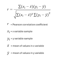
1. Generate a Correlation Matrix:
   • If you have multiple data columns, the correlation matrix will show the Pearson correlation for every pair of columns.
2. Create a Heatmap for Visualization:
   • A correlation heatmap will help visualize the strength and direction of correlations between variables.

VBA Code for Correlation Analysis:

Option Explicit
' This function calculates the Pearson correlation between two arrays of data.
Function PearsonCorrelation(arrX As Range, arrY As Range) As Double
    Dim i As Long
    Dim n As Long
    Dim sumX As Double, sumY As Double
    Dim sumXY As Double, sumX2 As Double, sumY2 As Double
    Dim correlation As Double
    n = arrX.Count
    If n <> arrY.Count Then
        MsgBox "Ranges must have the same number of rows.", vbCritical
        Exit Function
    End If
    ' Initializing sums
    sumX = 0
    sumY = 0
    sumXY = 0
    sumX2 = 0
    sumY2 = 0
    ' Loop through each value and compute the sums required for Pearson's formula
    For i = 1 To n
        sumX = sumX + arrX.Cells(i, 1).Value
        sumY = sumY + arrY.Cells(i, 1).Value
        sumXY = sumXY + arrX.Cells(i, 1).Value * arrY.Cells(i, 1).Value
        sumX2 = sumX2 + arrX.Cells(i, 1).Value ^ 2
        sumY2 = sumY2 + arrY.Cells(i, 1).Value ^ 2
    Next i
    ' Pearson Correlation formula
    correlation = (n * sumXY - sumX * sumY) / _
                  Sqr((n * sumX2 - sumX ^ 2) * (n * sumY2 - sumY ^ 2))
    PearsonCorrelation = correlation
End Function

' This subroutine calculates the correlation matrix for a range of columns.
Sub CorrelationMatrixAnalysis()
    Dim dataRange As Range
    Dim i As Long, j As Long
    Dim numColumns As Long
    Dim correlationResult As Double
    Dim matrixRange As Range   
    ' Specify the data range (assume data starts in cell A1)
    Set dataRange = Range("A1").CurrentRegion
    numColumns = dataRange.Columns.Count
    ' Output header for the correlation matrix
    With dataRange.Worksheet
        ' Set header for correlation matrix
        Set matrixRange = .Range("G1").Resize(numColumns, numColumns)
        matrixRange.Cells(1, 1).Value = "Correlation Matrix"       
        ' Loop through each combination of columns to calculate Pearson correlation
        For i = 1 To numColumns
            For j = 1 To numColumns
                ' Skip diagonal elements (correlation of a column with itself is always 1)
                If i = j Then
                    matrixRange.Cells(i + 1, j + 1).Value = 1
                Else
                    ' Calculate Pearson correlation between columns i and j
                    correlationResult = PearsonCorrelation(dataRange.Columns(i), dataRange.Columns(j))
                    matrixRange.Cells(i + 1, j + 1).Value = correlationResult
                End If
            Next j
        Next i
    End With
    MsgBox "Correlation Matrix Calculated Successfully"
End Sub

' This subroutine creates a color-coded heatmap for the correlation matrix.
Sub CreateHeatmap()
    Dim matrixRange As Range
    Dim cell As Range
    Dim correlationValue As Double
    Dim color As Long   
    ' Set the range for the correlation matrix (output from CorrelationMatrixAnalysis)
    Set matrixRange = Range("G2").CurrentRegion   
    ' Loop through each cell in the matrix and color based on correlation value
    For Each cell In matrixRange
        correlationValue = cell.Value       
        ' Apply colors based on correlation value
        If correlationValue > 0.8 Then
            color = RGB(0, 255, 0) ' Green for high positive correlation
        ElseIf correlationValue > 0.5 Then
            color = RGB(255, 255, 0) ' Yellow for moderate positive correlation
        ElseIf correlationValue < -0.8 Then
            color = RGB(255, 0, 0) ' Red for high negative correlation
        ElseIf correlationValue < -0.5 Then
            color = RGB(255, 165, 0) ' Orange for moderate negative correlation
        Else
            color = RGB(200, 200, 200) ' Gray for weak correlation
        End If       
        cell.Interior.Color = color
    Next cell
    MsgBox "Heatmap Created Successfully"
End Sub

Detailed Explanation of the Code:

1. PearsonCorrelation Function:
   • This function computes the Pearson correlation coefficient for two data ranges (arrays).
   • It checks if the data ranges have the same number of rows.
   • It calculates the required sums (sum of X, sum of Y, sum of XY, sum of X^2, and sum of Y^2).
   • It then uses these sums to compute the Pearson correlation using the Pearson correlation formula.
2. CorrelationMatrixAnalysis Subroutine:
   • This subroutine calculates the correlation matrix for a set of data columns.
   • The data range is assumed to start from cell A1 and covers all adjacent rows and columns.
   • The code loops through each pair of columns in the dataset, computes the correlation for each pair using the PearsonCorrelation function, and stores the result in a new range (starting at G1).
   • The diagonal elements (correlations of a column with itself) are set to 1, as the correlation of a variable with itself is always 1.
3. CreateHeatmap Subroutine:
   • This subroutine applies a color code to the correlation matrix based on the correlation values.
   • It uses green for strong positive correlations (greater than 0.8), red for strong negative correlations (less than -0.8), and various shades for other levels of correlation.
   • The heatmap provides a visual representation of the correlation strengths between data columns.

Usage:

1. Running the Analysis:
   • Open Excel and press ALT + F11 to open the VBA editor.
   • Insert a new module, and paste the code into it.
   • To run the analysis, press F5 while the CorrelationMatrixAnalysis or CreateHeatmap subroutine is selected.
2. Input Data:
   • The data should be organized in columns, where each column represents a different variable or dataset.
   • The code will compute the correlations between these variables.
3. Output:
   • The correlation matrix will be placed in a new range starting from cell G1.
   • The heatmap will color-code the matrix based on correlation strength.

Conclusion:

This advanced VBA code allows you to calculate and visualize correlations between multiple datasets in Excel. It is highly customizable, and you can extend it further by including other correlation types (e.g., Spearman’s rank correlation) or adding more visualization features. The heatmap is particularly useful for visually identifying strong relationships between variables.

Implementing advanced data compression techniques in Excel VBA can be a highly sophisticated task, but it’s definitely doable. Excel VBA doesn’t have built-in methods for compression like those found in specialized libraries such as zlib, but we can still implement rudimentary data compression algorithms, like Huffman coding or Run-Length Encoding (RLE), using VBA.

I’ll go over an example of how to implement Run-Length Encoding (RLE), a simple compression technique, in VBA. We’ll then discuss how it works and how you could expand this approach to implement more complex techniques like Huffman coding.

What is Run-Length Encoding (RLE)?

Run-Length Encoding (RLE) is a simple form of data compression in which consecutive elements (or « runs ») of the data that are the same are stored as a single value and count. For example, if you have the sequence:

AAAABBBCCDAA

It would be compressed to:

4A3B2C1D2A

The compression works because we replace each series of identical characters with the count of the characters followed by the character itself.

Step-by-Step Code for Run-Length Encoding (RLE) in VBA

Let’s start with a simple VBA function to compress a string using RLE.

Step 1: Open the VBA Editor

Press Alt + F11 to open the Visual Basic for Applications (VBA) editor in Excel.

Step 2: Insert a Module

• Right-click on VBAProject (Your Workbook Name) in the left-hand pane.
• Select Insert → Module.

Step 3: Write the Compression Code (RLE)

Function RunLengthEncode(inputStr As String) As String
    Dim outputStr As String
    Dim count As Integer
    Dim currentChar As String
    Dim i As Integer   
    ' Initialize output string
    outputStr = ""   
    ' Ensure the input string is not empty
    If Len(inputStr) = 0 Then
        RunLengthEncode = ""
        Exit Function
    End If   
    ' Initialize the count for the first character
    count = 1
    currentChar = Mid(inputStr, 1, 1)   
    ' Loop through the input string starting from the second character
    For i = 2 To Len(inputStr)
        If Mid(inputStr, i, 1) = currentChar Then
            ' If current character matches the previous one, increase the count
            count = count + 1
        Else
            ' When characters no longer match, append the count and character to output
            outputStr = outputStr & count & currentChar
            ' Reset count and set currentChar to new character
            currentChar = Mid(inputStr, i, 1)
            count = 1
        End If
    Next i   
    ' Append the last set of character count and character to output
    outputStr = outputStr & count & currentChar   
    ' Return the compressed string
    RunLengthEncode = outputStr
End Function

Explanation of the Code:

1. Input and Initialization:
   • The function takes an inputStr as a parameter, which is the string to be compressed.
   • It initializes outputStr to store the compressed result, and count to track the number of consecutive identical characters.
2. Looping Through the String:
   • We start by comparing each character in the input string to the previous one. If they match, we increment the count.
   • When the characters differ, we append the current count and character to outputStr and reset the count for the new character.
3. Finalizing the Compression:
   • After the loop finishes, the last run of characters is appended to outputStr.
4. Return the Result:
   • The function finally returns the compressed string.

Step 4: Test the Compression Function

To test the function, you can call it in a worksheet cell or from another VBA function:

Sub TestRunLengthEncoding()
    Dim originalString As String
    Dim compressedString As String   
    ' Test string
    originalString = "AAAABBBCCDAA"   
    ' Call the RunLengthEncode function
    compressedString = RunLengthEncode(originalString)   
    ' Output result
    MsgBox "Original: " & originalString & vbCrLf & "Compressed: " & compressedString
End Sub

Step 5: Explanation of Output

If you run the above TestRunLengthEncoding macro, it will show a message box with:

Original: AAAABBBCCDAA

Compressed: 4A3B2C1D2A

Step 6: How to Expand This to More Advanced Compression

While Run-Length Encoding is a simple technique, it’s effective for certain types of data, especially where there are long sequences of repeated characters. For more complex compression methods like Huffman Coding, you’d need to implement a more advanced algorithm. Here’s a brief explanation of how Huffman Coding works and how you could implement it:

Huffman Coding Overview

Huffman coding is a widely used algorithm for lossless data compression. It assigns variable-length codes to input characters, with shorter codes assigned to more frequent characters. This minimizes the total space required for storage.

The implementation of Huffman Coding in VBA would be significantly more complex than Run-Length Encoding because it involves creating a frequency table for the characters, building a binary tree based on these frequencies, and then generating the codes. However, I can guide you through the implementation if you’re interested.

Potential Next Steps for Compression Algorithms:

1. Huffman Coding: Implement a frequency analysis of characters, build a binary tree (using priority queues), and generate the corresponding codes.
2. Lempel-Ziv-Welch (LZW): A dictionary-based algorithm used by file formats like .gif and .zip.
3. Deflate Algorithm: This is a combination of LZ77 and Huffman coding, used in .zip and .gzip files.

Conclusion

This example demonstrates a simple compression algorithm (Run-Length Encoding) implemented in Excel VBA. While this is a relatively basic technique, you can extend it to more advanced compression methods like Huffman coding or LZW with further research and understanding of the underlying algorithms. Let me know if you’d like to dive deeper into any of these techniques!

Implementing advanced data clustering techniques in Excel using VBA (Visual Basic for Applications) involves a number of steps, including data preprocessing, selecting an appropriate clustering algorithm, and then coding the algorithm in VBA. One of the most common clustering techniques used in data analysis is K-means clustering, which groups data into clusters based on their similarities.

In this detailed explanation, I’ll guide you through a K-means clustering implementation using VBA. If you’re familiar with Excel, you’ll be able to see how the algorithm can be applied to your datasets directly in a spreadsheet. Let’s break this down step by step.

Step 1: Preparing the Data

Before we start writing the VBA code for K-means clustering, we need to prepare the data in Excel. Assume that we have a dataset of numerical values (for simplicity, let’s assume a 2D dataset).

1. Dataset Structure: Imagine your data is structured in columns like this:
   • Column A: Feature 1
   • Column B: Feature 2

You want to apply the clustering algorithm to these features.

1. Number of Clusters (k): You will need to decide on the number of clusters (k). This could be inputted manually, or you can automate the selection process through different techniques, but for simplicity, let’s assume k is fixed.

Step 2: K-Means Clustering Algorithm

Here’s the basic idea behind the K-means clustering algorithm:

1. Initialize Centroids: Randomly select k data points as initial centroids.
2. Assign Points to Clusters: For each data point, calculate the distance from each centroid and assign the data point to the nearest centroid.
3. Recalculate Centroids: After assigning all points to clusters, recalculate the centroids as the mean of the points in each cluster.
4. Repeat: Repeat the assignment and centroid recalculation steps until convergence, meaning the centroids no longer change.

Step 3: Writing the VBA Code

Now, let’s move to the code.

1. Press Alt + F11 to open the VBA editor.
2. Insert a new Module: Go to Insert > Module in the VBA editor.

Here’s the code for implementing K-means clustering in VBA:

Sub KMeansClustering()
    Dim ws As Worksheet
    Dim dataRange As Range
    Dim k As Integer
    Dim maxIterations As Integer
    Dim points() As Variant
    Dim centroids() As Variant
    Dim assignments() As Integer
    Dim newCentroids() As Variant
    Dim i As Integer, j As Integer, iteration As Integer
    Dim minDist As Double, dist As Double
    Dim closestCentroid As Integer
    Dim sumX As Double, sumY As Double
    Dim count As Integer   
    ' Set parameters
    Set ws = ThisWorkbook.Sheets("Sheet1") ' Your worksheet name
    Set dataRange = ws.Range("A2:B100") ' Adjust data range
    k = 3 ' Number of clusters (adjust this)
    maxIterations = 100 ' Maximum number of iterations to avoid infinite loops   
    ' Load data into an array
    points = dataRange.Value   
    ' Initialize centroids (randomly pick k points)
    ReDim centroids(1 To k, 1 To 2) ' Assuming 2D data (x, y)
    Randomize
    For i = 1 To k
        centroids(i, 1) = points(Int((UBound(points, 1) - 1 + 1) * Rnd + 1), 1)
        centroids(i, 2) = points(Int((UBound(points, 1) - 1 + 1) * Rnd + 1), 2)
    Next i
    ' Initialize assignment array
    ReDim assignments(1 To UBound(points, 1))
    ' Main K-means loop
    For iteration = 1 To maxIterations
        ' Step 1: Assign points to the nearest centroid
        For i = 1 To UBound(points, 1)
            minDist = 1E+30 ' Set to a large number initially
            closestCentroid = -1
            For j = 1 To k
                dist = (points(i, 1) - centroids(j, 1)) ^ 2 + (points(i, 2) - centroids(j, 2)) ^ 2
                If dist < minDist Then
                    minDist = dist
                    closestCentroid = j
                End If
            Next j
            assignments(i) = closestCentroid
        Next i       
        ' Step 2: Recalculate centroids
        ReDim newCentroids(1 To k, 1 To 2)
        For i = 1 To k
            sumX = 0
            sumY = 0
            count = 0
            For j = 1 To UBound(points, 1)
                If assignments(j) = i Then
                    sumX = sumX + points(j, 1)
                    sumY = sumY + points(j, 2)
                    count = count + 1
                End If
            Next j
            If count > 0 Then
                newCentroids(i, 1) = sumX / count
                newCentroids(i, 2) = sumY / count
            Else
                ' If no points are assigned to a centroid, reinitialize it randomly
                newCentroids(i, 1) = points(Int((UBound(points, 1) - 1 + 1) * Rnd + 1), 1)
                newCentroids(i, 2) = points(Int((UBound(points, 1) - 1 + 1) * Rnd + 1), 2)
            End If
        Next i       
        ' Check for convergence (if centroids didn't change, break the loop)
        If Not CentroidsChanged(centroids, newCentroids) Then
            Exit For
        End If   
        ' Update centroids
        centroids = newCentroids
    Next iteration   
    ' Step 3: Output results
    ' Write the assignments back to the sheet
    For i = 1 To UBound(assignments, 1)
        ws.Cells(i + 1, 3).Value = assignments(i) ' Assign clusters to Column C
    Next i   
    ' Output centroids (if needed)
    For i = 1 To k
        ws.Cells(i + 1, 5).Value = "Centroid " & i
        ws.Cells(i + 1, 6).Value = centroids(i, 1)
        ws.Cells(i + 1, 7).Value = centroids(i, 2)
    Next i   
    MsgBox "K-means clustering complete!", vbInformation
End Sub

Function CentroidsChanged(ByRef oldCentroids As Variant, ByRef newCentroids As Variant) As Boolean
    Dim i As Integer
    For i = 1 To UBound(oldCentroids, 1)
        If oldCentroids(i, 1) <> newCentroids(i, 1) Or oldCentroids(i, 2) <> newCentroids(i, 2) Then
            CentroidsChanged = True
            Exit Function
        End If
    Next i
    CentroidsChanged = False
End Function

Step 4: Explanation of the Code

Let’s break down the code:

1. Set Parameters:
   • We specify the worksheet, the data range (assumed to be in columns A and B), and the number of clusters (k).
   • We also set a maximum number of iterations (maxIterations), which prevents infinite loops if convergence is not reached.
2. Loading Data:
   • We load the data from the selected range into a 2D array points.
3. Initializing Centroids:
   • The centroids are initially selected randomly from the dataset. For each cluster, we randomly select a point from the data as the initial centroid.
4. Main Loop:
   • For each iteration, we:
     1. Assign each data point to the nearest centroid based on Euclidean distance.
     2. Recalculate the centroids as the mean of the points assigned to them.
     3. Check for convergence: If the centroids haven’t changed after an iteration, we break out of the loop.
5. Output:
   • After clustering, the assignments (which cluster each data point belongs to) are written back to Column C.
   • The final centroids are written to columns E, F, and G.
6. Convergence Check:
   • The function CentroidsChanged compares the old centroids with the new ones to check if the centroids have changed. If not, the loop terminates early.

Step 5: Running the Code

• Once the code is written, go back to Excel and press Alt + F8 to run the macro KMeansClustering.
• The algorithm will perform clustering and populate the data with the cluster assignments.

Conclusion

This VBA implementation of K-means clustering in Excel demonstrates how you can apply a machine learning technique directly within the spreadsheet environment. You can adapt this code to more complex clustering tasks by adjusting the number of clusters, incorporating more features (columns), or even implementing other advanced clustering algorithms like hierarchical clustering or DBSCAN, though they would require more complex logic.

To implement advanced data clustering algorithms using Excel VBA, we can focus on algorithms such as K-Means Clustering and Hierarchical Clustering. These algorithms are used in machine learning for grouping similar data points together. Below, I will provide an example of how to implement a K-Means Clustering Algorithm in Excel VBA, along with detailed explanations of the process.

K-Means Clustering in Excel VBA

K-Means is one of the most popular clustering algorithms. The idea is to partition a set of data points into K clusters in which each data point belongs to the cluster with the nearest mean.

Overview of K-Means Algorithm Steps:

1. Initialize K cluster centroids randomly (or by some other method).
2. Assign each data point to the nearest centroid.
3. Recompute the centroids as the mean of the points in each cluster.
4. Repeat steps 2 and 3 until the centroids do not change or a stopping criterion is met.

Step-by-Step Implementation in Excel VBA:

1. Prepare Your Data

Let’s assume you have a dataset with 2 features (columns) in an Excel worksheet:

• Column A (X1) contains the first feature.
• Column B (X2) contains the second feature.

We’ll use K=3 clusters in this example.

2. Define the VBA Code

Here is the VBA code to implement the K-Means Clustering algorithm.

Sub KMeansClustering()
    ' Define variables
    Dim ws As Worksheet
    Dim dataRange As Range
    Dim dataPoints As Range
    Dim k As Integer
    Dim numPoints As Integer
    Dim centroids() As Variant
    Dim assignments() As Integer
    Dim newCentroids() As Variant
    Dim i As Integer, j As Integer
    Dim iterations As Integer
    Dim maxIterations As Integer
    Dim clusterIndex As Integer
    Dim minDist As Double
    Dim dist As Double
    Dim sumX As Double, sumY As Double
    Dim count As Integer   
    ' Set worksheet and data range
    Set ws = ThisWorkbook.Sheets("Sheet1")
    Set dataRange = ws.Range("A2:B100") ' Modify this range as needed
    numPoints = dataRange.Rows.Count   
    ' Initialize number of clusters (K) and max iterations
    k = 3 ' You can modify K to any number
    maxIterations = 100 ' Set a reasonable number of iterations   
    ' Initialize the assignments and centroids arrays
    ReDim assignments(1 To numPoints)
    ReDim centroids(1 To k, 1 To 2) ' Centroids for each cluster
    ReDim newCentroids(1 To k, 1 To 2) ' New centroids after recomputation   
    ' Step 1: Initialize the centroids randomly from the data points
    Randomize
    For i = 1 To k
        centroids(i, 1) = dataRange.Cells(Int(Rnd() * numPoints) + 1, 1).Value
        centroids(i, 2) = dataRange.Cells(Int(Rnd() * numPoints) + 1, 2).Value
    Next i   
    ' Step 2: Start the K-means loop
    iterations = 0
    Do While iterations < maxIterations
        ' Step 3: Assign each data point to the nearest centroid
        For i = 1 To numPoints
            minDist = -1
            For clusterIndex = 1 To k
                dist = (dataRange.Cells(i, 1).Value - centroids(clusterIndex, 1)) ^ 2 + _
                       (dataRange.Cells(i, 2).Value - centroids(clusterIndex, 2)) ^ 2
                If minDist = -1 Or dist < minDist Then
                    minDist = dist
                    assignments(i) = clusterIndex
                End If
            Next clusterIndex
        Next i       
        ' Step 4: Recompute the centroids
        For i = 1 To k
            sumX = 0
            sumY = 0
            count = 0
            For j = 1 To numPoints
                If assignments(j) = i Then
                    sumX = sumX + dataRange.Cells(j, 1).Value
                    sumY = sumY + dataRange.Cells(j, 2).Value
                    count = count + 1
                End If
            Next j
            If count > 0 Then
                newCentroids(i, 1) = sumX / count
                newCentroids(i, 2) = sumY / count
            End If
        Next i       
        ' Check for convergence (if centroids haven't changed)
        Dim converged As Boolean
        converged = True
        For i = 1 To k
            If centroids(i, 1) <> newCentroids(i, 1) Or centroids(i, 2) <> newCentroids(i, 2) Then
                converged = False
                Exit For
            End If
        Next i       
        If converged Then Exit Do       
        ' Update centroids for next iteration
        For i = 1 To k
            centroids(i, 1) = newCentroids(i, 1)
            centroids(i, 2) = newCentroids(i, 2)
        Next i       
        iterations = iterations + 1
    Loop   
    ' Output the results
    For i = 1 To numPoints
        ws.Cells(i + 1, 3).Value = assignments(i) ' Assign cluster labels in Column C
    Next i
    MsgBox "Clustering Complete!"   
End Sub

Explanation of the Code:

1. Variables and Setup:

• ws: The worksheet object where the data is stored.
• dataRange: The range containing the data points (e.g., Columns A and B).
• k: The number of clusters (K).
• centroids(): Array to store the centroids of the K clusters.
• assignments(): Array to store the cluster assignment for each data point.
• iterations: The number of iterations of the K-Means algorithm.
• maxIterations: The maximum number of iterations allowed before stopping.

2. Initial Random Centroids:

• We initialize the centroids randomly by selecting random points from the dataset.

3. Assigning Points to Clusters:

• For each data point, we compute the Euclidean distance to each centroid and assign the point to the nearest centroid.

4. Recomputing Centroids:

• After assigning all points to clusters, we recompute the centroids by averaging all the points in each cluster.

5. Convergence Check:

• If the centroids don’t change significantly between iterations, the algorithm stops. This is our convergence check.

6. Output:

• The resulting cluster assignments for each data point are written into Column C of the worksheet.

How to Run This Code:

1. Open Excel and press Alt + F11 to open the VBA editor.
2. Insert a new module (Insert > Module) and paste the code inside the module.
3. Close the editor and run the macro by pressing Alt + F8, selecting KMeansClustering, and clicking Run.

The algorithm will assign each data point to one of the three clusters, and the results will be displayed in Column C of the worksheet.

Conclusion:

The code above demonstrates how to implement the K-Means Clustering algorithm using Excel VBA. You can modify the number of clusters (K) or the data range as needed. The steps involve initializing random centroids, assigning points to clusters, and iterating until convergence is reached. This algorithm is essential for unsupervised machine learning tasks and is commonly used in various data science applications.

To implement an advanced data cleansing algorithm using Excel VBA, we need to address several tasks, such as removing duplicates, handling missing values, standardizing text, handling outliers, and converting data into a consistent format. Here, I’ll break down the key components of the data cleansing process and provide you with a detailed VBA code to perform these actions.

Key Steps in Data Cleansing

1. Removing Duplicate Rows: This step identifies and removes any duplicate rows based on selected columns or the entire dataset.
2. Handling Missing Data: Missing data (often represented as empty cells or specific placeholders like « N/A » or « null ») can be replaced, interpolated, or removed.
3. Standardizing Text: Data often needs to be standardized (e.g., capitalizing the first letter of each word, removing extra spaces, etc.).
4. Handling Outliers: Outliers are data points that deviate significantly from other observations. These can be identified and removed or replaced.
5. Formatting Data: Ensuring all data is in the correct format (dates, numbers, etc.) and ensuring there are no hidden characters or formatting issues.

Detailed VBA Code Implementation

Here’s the VBA code that implements these steps in a structured way.

Sub AdvancedDataCleansing()
    Dim ws As Worksheet
    Dim lastRow As Long
    Dim lastCol As Long
    Dim rng As Range
    Dim cell As Range
    Dim col As Integer
    Dim replaceValue As String
    Dim outlierThreshold As Double
    Dim i As Long
    ' Set the worksheet
    Set ws = ThisWorkbook.Sheets("Data") ' Change "Data" to your sheet's name
    ' Find the last row and column of the dataset
    lastRow = ws.Cells(ws.Rows.Count, 1).End(xlUp).Row
    lastCol = ws.Cells(1, ws.Columns.Count).End(xlToLeft).Column
    ' Step 1: Remove duplicates based on all columns
    Set rng = ws.Range(ws.Cells(1, 1), ws.Cells(lastRow, lastCol))
    rng.RemoveDuplicates Columns:=Application.Transpose(Application.Evaluate("ROW(1:" & lastCol & ")")), Header:=xlYes

    ' Step 2: Handle missing data (blanks or placeholders like "N/A" or "null")
    For col = 1 To lastCol
        For Each cell In ws.Range(ws.Cells(2, col), ws.Cells(lastRow, col))
            If IsEmpty(cell.Value) Or cell.Value = "N/A" Or cell.Value = "null" Then
                ' Replace missing value with an appropriate value
                ' Here we replace with the word "Missing"
                cell.Value = "Missing" ' You can replace this with another value like "0" or "Unknown"
            End If
        Next cell
    Next col
    ' Step 3: Standardize text formatting (remove extra spaces, capitalize properly)
    For col = 1 To lastCol
        For Each cell In ws.Range(ws.Cells(2, col), ws.Cells(lastRow, col))
            If VarType(cell.Value) = vbString Then
                ' Trim spaces
                cell.Value = Trim(cell.Value)
                ' Capitalize each word
                cell.Value = Application.WorksheetFunction.Proper(cell.Value)
            End If
        Next cell
    Next col
    ' Step 4: Handle outliers in numeric data columns (assume numeric columns are of interest)
    ' Assuming we define an outlier as a value that is more than 2 standard deviations from the mean
    outlierThreshold = 2 ' This represents 2 standard deviations; change it to suit your needs
    For col = 1 To lastCol
        If IsNumeric(ws.Cells(2, col).Value) Then ' Check if the column contains numeric data
            ' Calculate mean and standard deviation
            Dim data As Range
            Set data = ws.Range(ws.Cells(2, col), ws.Cells(lastRow, col))
            Dim mean As Double, stdev As Double
            mean = Application.WorksheetFunction.Average(data)
            stdev = Application.WorksheetFunction.StDev(data)
            ' Check and clean outliers
            For Each cell In data
                If Abs(cell.Value - mean) > outlierThreshold * stdev Then
                    ' Replace outlier with the mean value (or another strategy)
                    cell.Value = mean
                End If
            Next cell
        End If
    Next col
    ' Step 5: Ensure consistent formatting (e.g., convert date columns to proper date format)
    For col = 1 To lastCol
        For Each cell In ws.Range(ws.Cells(2, col), ws.Cells(lastRow, col))
            If IsDate(cell.Value) Then
                ' Force the cell to follow a standard date format (MM/DD/YYYY)
                cell.NumberFormat = "mm/dd/yyyy"
            End If
        Next cell
    Next col
    MsgBox "Data Cleansing Complete", vbInformation
End Sub

Explanation of Each Step

Step 1: Remove Duplicates

The RemoveDuplicates method is used to remove duplicate rows based on all columns. You can adjust the columns argument if you only want to check specific columns for duplicates.

rng.RemoveDuplicates Columns:=Application.Transpose(Application.Evaluate("ROW(1:" & lastCol & ")")), Header:=xlYes

Step 2: Handle Missing Data

This step checks each cell for missing values (blank cells or placeholders like « N/A » or « null ») and replaces them with a chosen value. In this case, we’re replacing them with « Missing. »

If IsEmpty(cell.Value) Or cell.Value = "N/A" Or cell.Value = "null" Then
    cell.Value = "Missing"
End If

Step 3: Standardize Text Formatting

This part of the code trims any leading/trailing spaces from text values and capitalizes the first letter of each word in the cell.

If VarType(cell.Value) = vbString Then
    cell.Value = Trim(cell.Value)
    cell.Value = Application.WorksheetFunction.Proper(cell.Value)
End If

Step 4: Handle Outliers

For each numeric column, the mean and standard deviation are calculated. Outliers are defined as values more than 2 standard deviations away from the mean. Outliers are then replaced with the mean value.

If Abs(cell.Value - mean) > outlierThreshold * stdev Then
    cell.Value = mean
End If

Step 5: Consistent Formatting for Dates

This step ensures that date columns are correctly formatted as dates (MM/DD/YYYY in this example).

If IsDate(cell.Value) Then
    cell.NumberFormat = "mm/dd/yyyy"
End If

Additional Notes

• Handling other data types: You can add additional checks for other data types like numbers, currencies, etc., and apply any necessary formatting or replacements.
• Customizing thresholds: The threshold for outlier detection (e.g., 2 standard deviations) and the handling of missing data can be customized based on your specific use case.

Conclusion

This VBA script provides a robust starting point for cleansing your data in Excel. By automating the process of removing duplicates, handling missing values, standardizing text, addressing outliers, and formatting data consistently, you can significantly improve the quality of your dataset. You can further enhance this script to cater to more specific requirements as needed.

Step 1: Open Excel and Press Alt + F11 to Open the VBA Editor

1. Open Excel on your computer.
2. Press Alt + F11 to open the VBA Editor.
3. In the VBA Editor, you’ll write your anonymization code.

Step 2: Write VBA Code for Anonymization

In this step, we’ll create a macro that anonymizes sensitive data in Excel, such as names, phone numbers, email addresses, etc. There are many techniques you can use for data anonymization, but here we’ll demonstrate a few common techniques:

• Shuffling: Randomly shuffling the values in a column (e.g., shuffling names or phone numbers).
• Masking: Replacing values with a pattern (e.g., replacing digits with X).
• Generalization: Changing the values to a more general category (e.g., age ranges).
• Data Perturbation: Adding or subtracting a small amount of noise to make data slightly inaccurate while preserving its utility.

Sample Anonymization Techniques:

1. Shuffling Column Data (Randomize Rows)

This technique involves randomizing the order of data in a column, which anonymizes it without changing the values.

Explanation of the code:

• The ShuffleData macro randomizes the values in the specified range (from A2:A100 in this example).
• We load the data into an array, shuffle the array randomly, and then write it back to the original range.
• Rnd generates a random number between 0 and 1, and Int is used to ensure it’s a whole number, ensuring randomness.

2. Masking Data (Replace with « X »)

For sensitive information like phone numbers or email addresses, you may want to replace some or all digits with an X to maintain anonymity

Sub MaskData() 
Dim rng As Range 
Dim cell As Range 
Dim maskedValue As String 
' Define the range with the data to mask (Assuming data is in Column B) 
Set rng = Range("B2:B100") ' Loop through each cell in the range For Each cell In rng 
' Mask the data (replace each character with 'X') 
maskedValue = String(Len(cell.Value), "X") 
cell.Value = maskedValue Next cell 
End Sub

Explanation of the code:

• This macro loops through each cell in the defined range (B2:B100) and replaces the entire value with X characters, preserving the length of the original data.

3. Generalizing Data (Age to Age Range)

Instead of keeping exact ages, you might want to generalize them into ranges (e.g., « 20-30 », « 30-40 »).

Sub GeneralizeData()
    Dim rng As Range
    Dim cell As Range
    Dim age As Integer
    Dim ageRange As String   
    ' Define the range containing age data (Assuming ages are in Column C)
    Set rng = Range("C2:C100")   
    ' Loop through each cell and generalize the age
    For Each cell In rng
        age = cell.Value
        If age < 20 Then
            ageRange = "Under 20"
        ElseIf age >= 20 And age < 30 Then
            ageRange = "20-29"
        ElseIf age >= 30 And age < 40 Then
            ageRange = "30-39"
        ElseIf age >= 40 And age < 50 Then
            ageRange = "40-49"
        Else
            ageRange = "50+"
        End If
        ' Replace the exact age with the generalized range
        cell.Value = ageRange
    Next cell
End Sub

Explanation of the code:

• This macro loops through each cell in the C2:C100 range and assigns an age range based on the value.
• It replaces the exact age with a more general description, such as « 20-29 » or « 30-39 ».

4. Data Perturbation (Adding Noise)

For numerical data, you can add slight perturbations (noise) to ensure the data is anonymized while keeping it useful.

Sub PerturbData()
    Dim rng As Range
    Dim cell As Range
    Dim noise As Double
    Dim originalValue As Double   
    ' Define the range with numeric data (Assuming data is in Column D)
    Set rng = Range("D2:D100")
    
    ' Loop through each cell in the range
    For Each cell In rng
        originalValue = cell.Value
        ' Add random noise between -5% and 5% of the original value
        noise = originalValue * (Rnd - 0.5) * 0.1
        cell.Value = originalValue + noise
    Next cell
End Sub

Explanation of the code:

• This macro adds random noise to each value in the range.
• The noise is between -5% and +5% of the original value, preserving the data’s general trend but anonymizing it slightly.

Step 3: Run the Macro

To run the macro in Excel:

1. After you have written the code in the VBA editor, you can close the editor and go back to the Excel workbook.
2. Press Alt + F8 to open the Macro dialog box.
3. Select the macro you want to run (e.g., ShuffleData, MaskData, etc.).
4. Click Run.

The macro will execute, and you’ll see the anonymized data in the selected range.

---

Example Output:

Let’s say you have the following data in Column A (Name), Column B (Phone Number), and Column C (Age):

Name	Phone Number	Age
John Doe	123-456-7890	28
Jane Smith	234-567-8901	35
Bob White	345-678-9012	42

After running the Shuffling macro on Column A, the data might look like this:

Name	Phone Number	Age
Bob White	123-456-7890	28
John Doe	234-567-8901	35
Jane Smith	345-678-9012	42

After running the Masking macro on Column B, the data will be:

Name	Phone Number	Age
John Doe	XXXXXXXXXXXX	28
Jane Smith	XXXXXXXXXXXX	35
Bob White	XXXXXXXXXXXX	42

After running the Generalization macro on Column C, the data will become:

Name	Phone Number	Age
John Doe	XXXXXXXXXXXX	20-29
Jane Smith	XXXXXXXXXXXX	30-39
Bob White	XXXXXXXXXXXX	40-49

---

Conclusion:

By implementing these anonymization techniques in Excel VBA, you can protect sensitive data while keeping it useful for analysis. This ensures privacy while retaining the value of the data for further processing or reporting.