Votre panier est actuellement vide !
Étiquette : macro-ranges
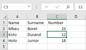
Sorting Cell Ranges in Excel with VBA
The Sort() method of the Range object allows for flexible sorting of data in Excel. It can be applied to sort by one or more sort keys (columns), and optionally take headers into account.
Later, a more complex example shows how to sort by more than three keys using the worksheet’s Sort object.
- Sorting by a Single Column (e.g., “Number”)
Sub SortingNummer()
    ThisWorkbook.Worksheets("Tabelle4").Activate
    Range("A1:C4").Sort Key1:=Range("C1:C4"), Header:=xlYes
End Sub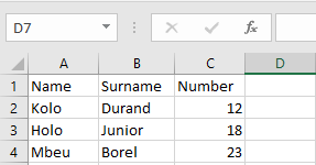
Explanation:
- Range(« A1:C4 ») defines the full data table.
- Key1:=Range(« C1:C4 ») tells Excel to sort by column C (e.g., Number).
- Header:=xlYes indicates that the first row is a header and should not be included in sorting.
- Order1 (ascending or descending) is optional. Default is ascending (xlAscending).
- Sorting by Two Columns (e.g., Last Name, then First Name)
Sub SortierenName()
    ThisWorkbook.Worksheets("Tabelle4").Activate
    Range("A1:C4").Sort Key1:=Range("A1:A4"), _
                        Key2:=Range("B1:B4"), Header:=xlYes
End Sub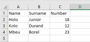
Explanation:
- Sorts first by Last Name (Column A), then by First Name (Column B).
- Up to three keys can be specified (Key1, Key2, Key3) with corresponding sort orders (Order1, Order2, Order3).
- Each key is processed in priority order.
- Sorting by More Than Three Keys
To sort with more than three criteria, use the SortFields collection of the worksheet’s Sort object.
Sub SortierenVieleSchluessel()
    ThisWorkbook.Worksheets("Tabelle5").Activate
    ' Clear old sort settings
    ActiveSheet.Sort.SortFields.Clear
    ' Add up to five sort keys
    ActiveSheet.Sort.SortFields.Add Range("A1:A6")
    ActiveSheet.Sort.SortFields.Add Range("B1:B6")
    ActiveSheet.Sort.SortFields.Add Range("C1:C6")
    ActiveSheet.Sort.SortFields.Add Range("D1:D6")
    ActiveSheet.Sort.SortFields.Add Range("E1:E6")
    ' Define the full range to be sorted
    ActiveSheet.Sort.SetRange Range("A1:E6")
    ' Apply the sorting
    ActiveSheet.Sort.Apply
End Sub
Explanation:
- .SortFields.Clear removes any previous sort configuration.
- .SortFields.Add adds each column that will serve as a sorting key.
- .SetRange(…) defines the total area of data to sort.
- .Apply executes the sort operation.
- By default, sorting is ascending. To specify order, add parameters to .Add, like:
- .Add Key:=Range(« A1:A6 »), Order:=xlDescending
Summary
Feature VBA Method Notes Sort one or two columns Range().Sort Use Key1, Key2, Header, optional Order1 Sort more than 3 columns ActiveSheet.Sort.SortFields Add fields with .Add(), finalize with .Apply() Header row Header:=xlYes Prevents header from being sorted Order (optional) Order:=xlAscending / xlDescending Can be added per key Clear old sort settings .Sort.SortFields.Clear Resets sort configuration Using the Offset Property in Excel VBA
The Offset property allows you to define a cell or range that is shifted relative to another. This offset can be applied to both individual cells and cell ranges — contiguous or non-contiguous.
The result of an Offset is always another Range object, which you can use to write, read, or format data.
Example:
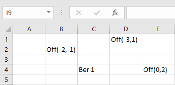
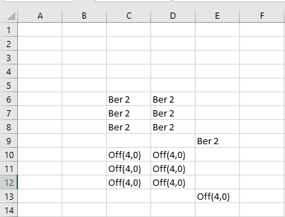
Sub cellOffset()
    ThisWorkbook.Worksheets("Sheet3").Activate
    ' Base cell = Cells(4, 3) = C4
    Cells(4, 3).Value = "Ber 1"
    Cells(4, 3).Offset(0, 2).Value = "Off(0,2)"     ' E4
    Cells(4, 3).Offset(-3, 1).Value = "Off(-3,1)"   ' D1
    Cells(4, 3).Offset(-2, -1).Value = "Off(-2,-1)" ' B2
    ' Offset of a range (non-contiguous: C6:D8 and E9)
    Range("C6:D8,E9").Value = "Ber 2"
    Range("C6:D8,E9").Offset(4, 0).Value = "Off(4,0)" ' Shifted down by 4 rows
    ' Offset-relative referencing (within E4, using A1-style notation)
    Cells(4, 3).Offset(0, 2).Range("A2").Value = "A2"
    Cells(4, 3).Offset(0, 2).Range("A3").Value = "A3"
    Cells(4, 3).Offset(0, 2).Range("B1").Value = "B1"
    Cells(4, 3).Offset(0, 2).Range("B2").Value = "B2"
    Cells(4, 3).Offset(0, 2).Range("B3").Value = "B3"
End Sub
Detailed Explanation:
- Basic Offset Calculation
When using:
Cells(4, 3) ‘ Refers to cell C4 (Row 4, Column 3)
The Offset(rowOffset, columnOffset) method returns a cell (or range) relative to this base:
- Rows are counted first (positive = down, negative = up)
- Columns are counted second (positive = right, negative = left)
Example Calculations:
- Cells(4, 3).Offset(0, 2) → Row 4 + 0, Column 3 + 2 = Cell E4
- Cells(4, 3).Offset(-3, 1) → Row 1, Column 4 = Cell D1
- Cells(4, 3).Offset(-2, -1) → Row 2, Column 2 = Cell B2
- Offset Applied to Ranges
Range(« C6:D8,E9 »).Offset(4, 0)
This example shows that Offset can also be applied to multiple-area ranges (even non-contiguous). It shifts the entire area 4 rows downward but keeps the shape and relative position of the original blocks.
So:
- C6:D8 becomes C10:D12
- E9 becomes E13
- Offset-Relative Cell References (Using A1 Notation)
When you use:
Cells(4, 3).Offset(0, 2).Range(« A2 »)
You’re accessing a cell relative to the top-left cell of the offset (in this case, E4):
- « A2 » refers to the cell 1 row down, same column within the new range (i.e., E5)
- « B3 » refers to 2 rows down, 1 column to the right (i.e., F6)
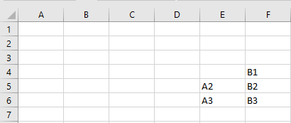
This technique allows you to work with relative cell references inside a shifted anchor cell — very useful for table structures, templates, and loops.
Summary
- Offset shifts a cell or range by a specified number of rows and columns.
- It returns a new Range object — ideal for positioning content programmatically.
- You can apply it to individual cells, entire ranges, and even multi-area ranges.
- Use .Range(« A1 »)-style references relative to the offset anchor for fine control inside dynamic areas.
Detecting Special Cells in Excel VBA
The SpecialCells() method in Excel VBA is a powerful tool for identifying specific types of cells within a range. Once identified, these cells can be visually highlighted or processed individually.
The following VBA procedure demonstrates how to:
- Highlight all cells that contain formulas
- Highlight all empty (blank) cells
- Identify and highlight the last used cell in the worksheet
VBA Code Example:
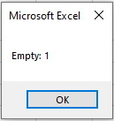
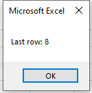
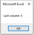
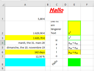
Sub Special cells()
    ThisWorkbook.Worksheets("Sheet2").Activate
    ' Cells with formulas
    Range("A1:A8").SpecialCells(xlCellTypeFormulas).Interior.Color = vbYellow
    MsgBox "Formulas: " & Range("A1:A9").SpecialCells(xlCellTypeFormulas).Count
    ' Empty (blank) cells
    Range("A1:A8").SpecialCells(xlCellTypeBlanks).Interior.Color = vbCyan
    MsgBox "Empty: " & Range("A1:A8").SpecialCells(xlCellTypeBlanks).Count
    ' Last used cell in the worksheet
    ActiveSheet.UsedRange.SpecialCells(xlCellTypeLastCell).Interior.Color = vbGreen
    MsgBox "Last row: " & ActiveSheet.UsedRange.SpecialCells(xlCellTypeLastCell).Row
    MsgBox "Last column: " & ActiveSheet.UsedRange.SpecialCells(xlCellTypeLastCell).Column
End Sub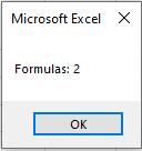
Detailed Explanation:
The SpecialCells() Method
This method returns a Range object containing only the cells that match the specified condition within a given range.
Common Constants:
- xlCellTypeFormulas: returns only the cells that contain formulas
- xlCellTypeBlanks: returns all empty cells (no value and no formula)
- xlCellTypeLastCell: returns the last cell in the used range, based on formatting and content
How the Code Works:
Cells with formulas:
Range(« A1:A8 »).SpecialCells(xlCellTypeFormulas)
-
- Finds all cells in A1:A8 that contain formulas
- Highlights them with yellow
- Displays the count in a message box
Blank (empty) cells:
Range(« A1:A8 »).SpecialCells(xlCellTypeBlanks)
-
- Finds all empty cells in the range
- Highlights them with cyan
- Shows the number of blank cells in a message box
Last used cell in the worksheet:
UsedRange.SpecialCells(xlCellTypeLastCell)
-
- Identifies the last non-empty or formatted cell on the active worksheet
- Highlights it with green
- Displays its row and column number using .Row and .Column
Note:
- UsedRange refers to the smallest rectangle that includes all non-empty or formatted cells.
- The last used cell may not always be where the last visible value is — formatting or deleted values may extend it.
- For a multi-cell range, properties like .Row or .Column return the top-left cell’s position in that range:
- Example:
- Range(« A3:B5 »).Row ‘ returns 3
- Range(« A3:B5 »).Column ‘ returns 1
Summary
- SpecialCells() is ideal for targeting only relevant cells (formulas, blanks, constants, etc.).
- Use it for conditional formatting, data validation, or auditing worksheets.
- Always handle potential errors: if no matching cells exist, SpecialCells() will raise an error unless handled with On Error Resume Next..
Setting Row Height and Column Width in Excel VBA
The following VBA procedure sets the height of specific rows and the width of specific columns:
Sub SetRowHeightAndColumnWidth()
    ' Activate the worksheet named "Sheet1"
    ThisWorkbook.Worksheets("Sheet1").Activate
    ' Set the height of rows 1 and 2 to 55 points
    Range("1:2").RowHeight = 55
    ' Set the width of columns B and D to 3 characters
    Range("B:B,D:D").ColumnWidth = 3
End Sub
Detailed Explanation:
This procedure adjusts the layout of the worksheet by modifying:
- Row height for rows 1 and 2.
- Column width for columns B and D.
RowHeight Property
The RowHeight property specifies the height of the row(s) in points.
In this example:Range(« 1:2 »).RowHeight = 55
This sets the height of rows 1 and 2 to 55 points.
ColumnWidth Property
The ColumnWidth property determines the width of the column(s).
Column width is based on the number of characters of the default font that can fit in a cell.In this case:
Range(« B:B,D:D »).ColumnWidth = 3
This sets the width of columns B and D to 3 characters, which is relatively narrow.
AutoFit Method: Adjusting Size Automatically
If you want Excel to automatically adjust the row height or column width based on the content, use the .AutoFit method.
Examples:
- To auto-adjust column G:
- Range(« G:G »).Columns.AutoFit
- To auto-adjust rows 1 and 2:
- Range(« 1:2 »).Rows.AutoFit
This is particularly useful when you’re not sure of the required size and want the dimensions to match the content exactly.
Summary
- RowHeight sets row height in points.
- ColumnWidth sets column width in character units.
- Use .AutoFit for automatic sizing based on content.
Identifying the Used Cell Range in Excel VBA
In Excel VBA, the UsedRange property is a very useful feature of a worksheet. It refers to the smallest rectangular block of cells that includes all non-empty or formatted cells on the sheet.
However, there’s a common caveat:
Not all used cells visibly contain content. For example:- If a cell previously contained a value (like a date) and the value was later deleted, the formatting (e.g., date format) might still remain.
- Excel considers any formatted cell (even if visually empty) as part of the UsedRange.
So, from a programming perspective, even an « empty » worksheet may have a non-empty UsedRange due to invisible formats or leftovers.
Tip:
If you want to ensure a clean slate before adding new data, consider clearing the worksheet completely using:Cells.Delete
Example: VBA to Highlight and Count Used Cells
The following procedure highlights all cells in the used range, colors them, and displays how many cells are considered « used »:
Sub HighlightUsedRange()
    ' Activate the worksheet named "Sheet1"
    ThisWorkbook.Worksheets("Sheet1").Activate
    ' Apply red borders to the used range
    ActiveSheet.UsedRange.Borders.Color = vbRed
    ' Apply yellow background color to the used range
    ActiveSheet.UsedRange.Interior.Color = vbYellow
    ' Display a message box showing the number of cells in the used range
    MsgBox "Count: " & ActiveSheet.UsedRange.Count
End Sub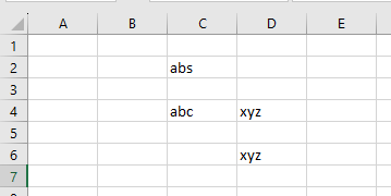
What This Procedure Does:
- Activates the worksheet named « Sheet1 ».
- Retrieves the UsedRange — the rectangular area that includes all non-empty or formatted cells.
- Adds a red border (vbRed) around the entire used range.
- Fills all used cells with a yellow background (vbYellow).
- Displays a message box showing how many individual cells are in the used range:
- MsgBox « Anzahl: » & ActiveSheet.UsedRange.Count

Key Concepts:
- UsedRange: Returns a Range object representing all used cells.
- .Borders.Color: Adds border color to all cells in the range.
- .Interior.Color: Sets the fill color of each cell in the range.
- .Count: Returns the number of individual cells in the range (not rows or columns).
Example:
Let’s say you only see values in a few scattered cells, but the UsedRange returns a larger rectangle — that’s because formatting remnants (like date, bold, etc.) still count as « usage ».
Summary
- UsedRange captures all non-empty or formatted cells.
- This may include seemingly « empty » cells if they retain formatting.
- Use .Count to determine how many cells are involved.
- Visually highlight the range to debug or understand your worksheet structure.
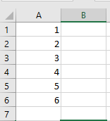
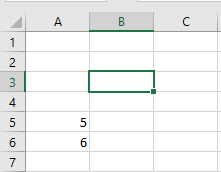
Deleting Cells and Rows in ExcelVBA
The following VBA procedure demonstrates how to delete specific cell ranges from a worksheet:
Sub DeleteCells()
    ' Activate the worksheet named "Tabelle1"
    ThisWorkbook.Worksheets("Sheet1").Activate
    ' Delete entire rows 6 and 7
    Range("6:7").Delete
    ' Delete cells A2 and A3, shifting the remaining cells upward
    Range("A2:A3").Delete Shift:=xlShiftUp
End Sub
Detailed Explanation:
The Delete Method
The Delete method of the Range object is used to remove cells, rows, or columns from a worksheet.
Optional Parameter: Shift
The Shift parameter defines how Excel rearranges neighboring cells after the deletion:
- xlShiftUp: shifts remaining cells upward to fill the gap
- xlShiftToLeft: shifts remaining cells left to fill the gap
If the Shift parameter is omitted, Excel determines the shifting direction based on the shape of the range:
- If the range is taller than wide, cells are typically shifted up.
- If the range is wider than tall, cells are typically shifted left.
What This Procedure Does:
- Activates the worksheet named « Tabelle1 ».
- Deletes entire rows 6 and 7 using:
- Range(« 6:7 »).Delete
Since full rows are selected, all rows below them are automatically shifted upward. The Shift parameter is not needed here.
- Deletes the cells in range A2:A3 using:
- Range(« A2:A3 »).Delete Shift:=xlShiftUp
This removes the two vertical cells and shifts the cells below them upward to fill the space.
Alternatively, Shift:=xlShiftToLeft would shift the neighboring cells to the left instead — useful for horizontal ranges.Additional Notes:
- To delete entire rows from a cell range:
- Range(« A2:A3 »).EntireRow.Delete
This would remove rows 2 and 3 entirely.
- To delete entire columns:
- Range(« A2:A3 »).EntireColumn.Delete
This would delete column A.
- This procedure effectively reverses the changes made by the previous insertion procedure (ZelleEinfuegen), returning the worksheet to its original structure.
Summary
- Use .Delete to remove cells, rows, or columns.
- Use Shift to control whether neighboring cells move up or left.
- For full rows or columns, Excel handles shifting automatically, and the Shift parameter is unnecessary.
Designing the Background Color of Cells in Excel VBA
The following VBA procedure is used to apply a background color to two specific cells — E2 and E6:

Sub ZellformatMuster()
    ThisWorkbook.Worksheets("Tabelle2").Activate
    Rane("E2, E6").Interior.Color = vbYellow
End Sub
Explanation:
Interior Property
The Interior property in Excel VBA is used to format the interior (or fill) of a cell or a range of cells. This includes settings like background color and pattern.
Key Sub-properties:
- Color – Defines the solid background color of the cell. You can assign:
- Predefined color constants, such as vbYellow, vbRed, vbBlue, vbGreen, etc.
- Or custom colors using the RGB() function, e.g.:
- Range(« A1 »).Interior.Color = RGB(255, 200, 0)
Note: In this example, the cells E2 and E6 are filled with yellow using the vbYellow constant.
Summary of What the Code Does:
- Activates the worksheet named « Tabelle2 ».
- Applies a yellow background color to cells E2 and E6.
If you’d like to go further (e.g., apply patterned fills or combine colors and patterns), you can also use the following Interior properties:
- Pattern: to set a fill pattern (e.g., xlGray16, xlSolid, xlUp, etc.)
- PatternColor: to define the color of the pattern itself
Example with pattern:
Range(« E2 »).Interior.Pattern = xlGray16
Range(« E2 »).Interior.PatternColor = vbRed
Range(« E2 »).Interior.Color = vbYellow
This fills the cell with a yellow background and overlays it with a red-gray pattern.
- Color – Defines the solid background color of the cell. You can assign:
Closes all open workbooks in Excel VBA
Here is a procedure that closes all open workbooks:
Sub CloseAllWorkbooks()
    Workbooks.Close
End Sub
Explanation:
TheClose()method is called on theWorkbooksobject. This closes all open workbooks but does not close the Visual Basic Editor (VBE) or Excel Help.
Excel itself remains open after running this procedure.
If a user has made changes to any workbook, they will be prompted to save those changes .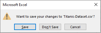
Deleting Cell Contents in Excel VBA
The following VBA procedure demonstrates how to delete specific parts of cell content from a worksheet—whether that be the content itself, the formatting, or everything including comments.
VBA Example: Clearing Different Aspects of Cell Content
Sub ClearCellContent()
    ThisWorkbook.Worksheets("Sheet1").Activate
    ' Clear everything: values, formatting, and comments
    Range("A1:A2").Clear
    ' Clear only the values; keep formatting and comments
    Range("A3:A4").ClearContents
    ' Clear only the formatting; keep values and comments
    Range("A5:A6").ClearFormats
End Sub
Explanation of the Procedure:
Worksheet Activation:
The macro begins by activating the « Sheet1 » worksheet to ensure all operations are targeted correctly.Clear() – Remove All:
Range(« A1:A2 »).Clear
-
- This removes everything from cells A1:A2:
- Cell values (data)
- Cell formatting (colors, fonts, borders, etc.)
- Any cell comments or notes
- This removes everything from cells A1:A2:
ClearContents() – Remove Only the Values:
Range(« A3:A4 »).ClearContents
-
- This deletes only the content (the actual data inside the cell).
- The cell’s appearance (formatting) and comments remain unchanged.
ClearFormats() – Remove Only the Formatting:
Range(« A5:A6 »).ClearFormats
-
- This deletes all formatting (like background colors, fonts, borders).
- The cell content (values) and comments remain untouched.
Visual Outcome:
- Before the Procedure Runs:
Cells contain values, colors, font styles, and possibly comments.
- After the Procedure Runs:
- A1:A2 are completely cleared—empty with default formatting.
- A3:A4 still look the same but are now empty (values are gone).
- A5:A6 retain their content, but their formatting resets to default .
Summary of Methods:
Method Removes… Clear() Values + Formatting + Comments ClearContents() Only Values ClearFormats() Only Formatting These tools help automate precise cleanup operations in worksheets, ideal when preparing data or resetting user inputs.
-
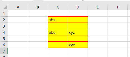
Framing Cell Ranges in Excel with VBA
The following VBA procedure shows how to apply borders to various cell ranges, either completely or partially:

Sub ZellformatRahmen()
    ThisWorkbook.Worksheets("Tabelle2").Activate
    Range("E2:E3").Borders.LineStyle = xlDouble
    Range("E2:E3").Borders.Weight = xlThick
    Range("E2:E3").Borders.Color = vbGreen
    Range("E4:E6").Borders(xlEdgeLeft).Weight = xlThin
    Range("E4:E6").Borders(xlEdgeRight).Weight = xlThin
    Range("E4:E6").Borders(xlInsideHorizontal).Weight = xlHairline
End Sub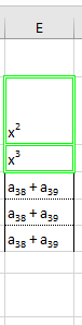
Explanation:
General Use of .Borders
The Borders property allows you to format the borders of a range in Excel. If you use Borders without a specific parameter (i.e., Range(…).Borders), the formatting will apply to all sides of the selected cell range — top, bottom, left, right, and all internal lines.
Targeting Specific Borders
To style only specific borders of a cell or range, you can specify one of the following border constants inside the Borders() method:
- xlEdgeLeft: Left border
- xlEdgeRight: Right border
- xlEdgeTop: Top border
- xlEdgeBottom: Bottom border
- xlInsideHorizontal: Inner horizontal lines (between rows)
- xlInsideVertical: Inner vertical lines (between columns)
If you only want to style the outer frame of a range, you must use constants beginning with xlEdge.
Styling Borders
You can modify different aspects of a border using the following properties:
- LineStyle – Defines the type of line used for the border:
- xlContinuous: solid line
- xlDot: dotted line
- xlDash: dashed line
- xlDouble: double line
- Others include xlDashDot, xlSlantDashDot, etc.
- Weight – Specifies the thickness of the border line. Accepted constants (from the xlBorderWeight enumeration):
- xlHairline: very thin line
- xlThin: thin line
- xlMedium: medium line
- xlThick: thick line
- Color – Determines the color of the border:
- Use predefined color constants like vbGreen, vbRed, vbBlue, etc.
- Or use the RGB() function for custom colors, e.g., RGB(255, 0, 0) for red.
Summary of What the Code Does:
- Activates the worksheet named « Tabelle2 ».
- Adds a double green thick border around the cells in E2:E3.
- For the range E4:E6, it adds:
- A thin left border (xlEdgeLeft)
- A thin right border (xlEdgeRight)
- And very thin horizontal lines (xlHairline) between the rows (xlInsideHorizontal)