Étiquette : macro-ranges

Formatting Individual Characters in a Cell with VBA

The following VBA procedure shows how to apply formatting to specific characters within a text string in Excel cells. This allows you to format subscripts, superscripts, or apply styles like bold or italic to only a part of the text in a cell—useful for scientific notation, equations, or special symbols.

VBA Example: Superscript and Subscript Formatting

Sub FormatIndividualCharacters()
    ThisWorkbook.Worksheets("Sheet2").Activate
    ' Add text to cells
    Range("E2").Value = "x2"
    Range("E3").Value = "x3"
    ' Superscript the second character (the number) in both cells
    Range("E2:E3").Characters(2, 1).Font.Superscript = True
    ' Add text to more cells
    Range("E4:E6").Value = "a38 + a39"
    ' Subscript "38" and "39" in all three cells
    Range("E4:E6").Characters(2, 2).Font.Subscript = True     ' Formats "38"
    Range("E4:E6").Characters(8, 2).Font.Subscript = True     ' Formats "39"
End Sub

Explanation of the Procedure:

Activate the Worksheet:

Ensures that « Sheet2 » is selected before applying changes.

Adding Content to Cells:

Range(« E2 »).Value = « x2 »

Range(« E3 »).Value = « x3 »

• • Two cells are filled with simple expressions (x2, x3).

Formatting with .Characters(start, length):

Range(« E2:E3 »).Characters(2, 1).Font.Superscript = True

• • This line targets the second character of the string (the number 2 or 3) in cells E2 and E3, and applies superscript formatting to it.
  • The syntax .Characters(start, length) allows you to select part of the string:
    • start: the position where formatting begins (1-based index)
    • length: how many characters to format

Working with Subscript Formatting:

Range(« E4:E6 »).Value = « a38 + a39 »

Range(« E4:E6 »).Characters(2, 2).Font.Subscript = True ‘ Targets « 38 »

Range(« E4:E6 »).Characters(8, 2).Font.Subscript = True ‘ Targets « 39 »

1. • Each of the cells E4 to E6 contains the text a38 + a39.
   • The two-character substrings « 38 » and « 39 » are subscripted by accessing:
     • Position 2, length 2 → « 38 »
     • Position 8, length 2 → « 39 »

Visual Outcome :

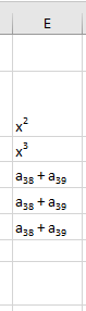
• E2 displays: x²
• E3 displays: x³
• E4 to E6 display: a₃₈ + a₃₉

Superscript is used for exponents, and subscript is used for variable indices—commonly seen in scientific and mathematical notation.

Key Concepts Recap:

Element	Purpose
.Characters(start, length)	Selects a part of the cell’s text
.Font.Superscript = True	Applies superscript to selected characters
.Font.Subscript = True	Applies subscript to selected characters

This technique allows precise formatting within cells—ideal for chemical formulas, math expressions, and technical documentation.

 

Setting Font Properties in Excel VBA

The following VBA procedure demonstrates how to customize the font formatting of a cell. You can define the font name, boldness, italic style, underline, size, and color using the Font object.

VBA Example: Formatting Cell Font

Sub FormatFontProperties()
    ' Activate the worksheet named "Tabelle2"
    ThisWorkbook.Worksheets("Tabelle2").Activate
    ' Set the font of cell C1 to Tahoma
    Range("C1").Font.Name = "Tahoma"
    ' Make the font bold
    Range("C1").Font.Bold = True
    ' Make the font italic
    Range("C1").Font.Italic = True
    ' Underline the font
    Range("C1").Font.Underline = True
    ' Set the font size to 20
    Range("C1").Font.Size = 20
    ' Set the font color to red
    Range("C1").Font.Color = vbRed
End Sub

Explanation of the Procedure:

1. Activating the Worksheet:
   • The procedure begins by activating « Sheet2 » to make sure all formatting changes apply to the correct sheet.
2. Using the Font Object:
   • Range(« C1 »).Font gives access to all font-related properties for cell C1.
   • Each property modifies a specific aspect of the cell’s text appearance.
3. Font Properties Used:

Property	Function	Example Value
.Name	Sets the font family	« Tahoma »
.Bold	Makes text bold if set to True	True or False
.Italic	Applies italic style	True or False
.Underline	Underlines the text	True or False
.Size	Sets the font size in points	20
.Color	Defines the font color	vbRed

You can simplify the syntax using a With block, as shown in the optimized version above.

Font Color Options:

• In the example, the color red is applied using the VBA color constant vbRed.
• Alternatively, you can use the RGB() function for custom colors:

• Range(« C1 »).Font.Color = RGB(255, 0, 0)

• • This sets the text color to red by specifying full red (255), and no green or blue (0).

Function/Constant	Description
vbRed	Built-in constant for red
RGB(r, g, b)	Custom color defined by RGB values

Result Overview:

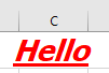
• Cell C1 displays the word « Hello » (or another value) using:
  • Tahoma font
  • Bold + Italic + Underlined
  • Font size: 20 pt
  • Font color: Red

Aligning Cells in Excel VBA

The following VBA procedure demonstrates how to align text horizontally and vertically, wrap long text, merge cells, and rotate text within a worksheet.

VBA Example: Aligning and Formatting Cells

Sub FormatCellAlignment()
    ThisWorkbook.Worksheets("Sheet2").Activate
    ' Center text horizontally and align it to the top vertically
    Range("C1").Value = "Hello"
    Range("C1").HorizontalAlignment = xlCenter
    Range("C1").VerticalAlignment = xlTop
    ' Wrap longer text within a single cell
    Range("C2").Value = "This is a longer piece of text"
    Range("C2").WrapText = True
    ' Merge multiple cells and display text vertically
    Range("C3").Value = "Hello"
    Range("C3:C7").MergeCells = True
    Range("C3:C7").Orientation = xlVertical
    ' Rotate text at an angle of 45 degrees
    Range("C8").Value = "Hello"
    Range("C8").Orientation = 45
End Sub

Explanation of the Procedure:

Activating the Worksheet:
The procedure starts by activating the worksheet named « Sheet2 ».

Horizontal and Vertical Alignment:

Range(« C1 »).HorizontalAlignment = xlCenter

Range(« C1 »).VerticalAlignment = xlTop

• • Aligns the text centered horizontally and top-aligned vertically.
  • Common constants for alignment:
    • Horizontal:
      • xlLeft → left-aligned
      • xlRight → right-aligned
      • xlCenter → centered
      • xlJustify → justified (blocks of text)
    • Vertical:
      • xlTop → aligned at the top
      • xlCenter → vertically centered
      • xlBottom → aligned at the bottom

Text Wrapping:

Range(« C2 »).WrapText = True

• • Enables automatic line breaks within the cell when the text is too long to fit.
  • If set to False, the text will remain on a single line, possibly overflowing beyond the cell’s edge.

Merging Cells and Displaying Text Vertically:

Range(« C3:C7 »).MergeCells = True

Range(« C3:C7 »).Orientation = xlVertical

• • Merges the cell range C3:C7 into one large cell.
  • Sets the text orientation to vertical, so the characters appear stacked one below the other.

Rotating Text at a Custom Angle:

Range(« C8 »).Orientation = 45

1. • Rotates the cell content to a 45-degree angle.
   • Orientation accepts:
     • Values from -90 to +90 degrees
     • The default is 0 (horizontal)
     • Special constant: xlVertical for vertical character stacking

Summary of Key Properties:

Property	Function
HorizontalAlignment	Aligns text left, center, right, or justified horizontally
VerticalAlignment	Aligns text top, center, or bottom vertically
WrapText	Enables/disables text wrapping within the cell
MergeCells	Merges or unmerges cell ranges
Orientation	Sets text direction (angle or vertical stacking)

Result Preview :

• C1: « Hello », centered horizontally and aligned to the top.
• C2: Long text that wraps into multiple lines.
• C3:C7: Merged block showing « Hello » vertically.
• C8: « Hello » displayed at a 45° angle.

 

The following VBA procedure shows how to apply custom number formats to cells, including formats for currency, dates, and percentages, using the NumberFormatLocal property.

VBA Example: Formatting Numbers, Dates, and Percentages

Sub CellFormatNumbers()
    ThisWorkbook.Worksheets("Sheet1").Activate
    ' Number with thousands separator, 2 decimals, and currency symbol
    Range("A1:A3").NumberFormat = "#,##0.00 €"
    ' Date: full weekday, "the", day, month, year
    Range("A4:A5").NumberFormat = "dddd, ""the"" dd. mmmm yy"
    ' Custom format: value followed by the word "days"
    Range("A6").NumberFormat = "0 ""days"""
    ' Percentage with 2 decimal places
    Range("A7").NumberFormat = "0.00 %"
End Sub

Explanation of the Procedure:

ThisWorkbook.Worksheets(« Sheet1 »).Activate
➡ Activates the worksheet named « Sheet1 » that belongs to the same workbook where the macro is saved (ThisWorkbook).
Make sure the sheet name is spelled exactly as it appears in Excel, or this line will trigger Run-time error ‘9’.

Range(« A1:A3 »).NumberFormat = « #,##0.00 € »
➡ Formats cells A1 to A3 as numbers:

• Thousands separator (,),
• Two decimal places,
• Euro currency symbol (€),

Example output: 1,629.90 €.

Range(« A4:A5 »).NumberFormat = « dddd, «  »the » » dd. mmmm yy »
➡ Formats dates in A4 and A5 to:

• Full weekday name (e.g., « Tuesday »),
• The word « the » (in quotation marks),
• Day number,
• Full month name,
• Two-digit year.

Example: Tuesday, the 31. March 20.

Range(« A6 »).NumberFormat = « 0 «  »days » » »
➡ Formats the value in cell A6 to display as a number followed by the word days:

Example: 142 days.

Range(« A7 »).NumberFormat = « 0.00 % »
➡ Formats A7 as a percentage with two decimal places:

• Example: 0.125 → 12.50 %.

Summary
This macro:

• Assumes data is in « Sheet1 »,
• Applies professional formatting for currency, dates, durations, and percentages,
• Helps make spreadsheet values easier to read and present.

 

The following VBA procedure shows how to insert numbers, dates, percentages, and formulas into specific cells on the worksheet named « Sheet2 ».

Note: Depending on your Excel setup, this sheet may not exist by default. If necessary, create it manually before running the code.

VBA Example: Assigning Values and Formulas

Sub ValuesAndFormulas()
    ThisWorkbook.Worksheets("Sheet2").Activate
    ' Numeric values
    Range("A1").Value = 5.8
    Range("A2").Value = 1629.9
    Range("A3").Formula = "=SUM(A1:A2)" ' English formula
    ' Date values
    Range("A4").Value = "2020/03/31"
    Range("A5").Value = "2019/11/10"
    Range("A6").Formula = "=A4-A5" ' Difference in days
    ' Percentage value
    Range("A7").Value = 0.125
End Sub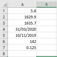

Explanation of the Procedure:

Activating the Worksheet:
The code starts by activating « Sheet2 » to make sure that the operations apply to the correct sheet.

Inserting Numeric Values:

Range(« A1 »).Value = 5.8

Range(« A2 »).Value = 1629.9

• • These lines insert decimal numbers into cells A1 and A2.
  • When assigning decimals in VBA, use a period (.) as the decimal separator regardless of your regional Excel settings.

Inserting a Formula (Localized Version):

Range(« A3 »).FormulaLocal = « =SUMME(A1:A2) »

• • This line adds a formula in cell A3 to sum the values in A1 and A2.
  • FormulaLocal is used so the formula can be written in the local language (German in this case). The result of the formula appears in the cell, and the formula remains visible in the formula bar.

Inserting Date Values:

Range(« A4 »).Value = « 2020/03/31 »

Range(« A5 »).Value = « 2019/11/10 »

• • Dates are input as text strings. Use double quotation marks around each date.
  • It’s recommended to use the US-style format (YYYY/MM/DD) for dates, as this is reliably recognized by VBA and avoids localization issues.
  • Excel will automatically interpret and format these as dates.

Calculating Date Difference:

Range(« A6 »).FormulaLocal = « =A4-A5 »

• • This formula computes the difference in days between the two dates in A4 and A5.
  • The result will be a numerical value representing the number of days between those dates.

Inserting a Percentage or Decimal Value:

Range(« A7 »).Value = 0.125

1. • This inserts a decimal number into A7, which can be formatted as a percentage in Excel (e.g., 12.5%) depending on cell formatting.

Result Overview:

After running this procedure (as shown in the referenced Figure 2.24):

• Cells A1 and A2 contain numeric values.
• A3 contains a formula that calculates their sum.
• A4 and A5 contain dates.
• A6 calculates the number of days between the two dates.
• A7 holds a decimal number (which could be used for percentages or ratios).

As explained earlier in Section 2.4.3 (« Moving or Copying Cell Contents »), it’s possible to copy the content of cells to the clipboard. This becomes especially useful when you want to copy only specific parts of a cell’s content—such as just the values or just the formats, rather than everything.

The following VBA example illustrates how to do exactly that:

VBA Example: Copying Only Values or Only Formats

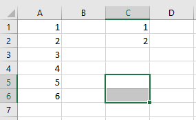
Sub CopyCellParts()
    ThisWorkbook.Worksheets("Sheet1").Activate
    ' Copy values only from A1:A2 to C1:C2
    Range("A1:A2").Copy
    Range("C1").PasteSpecial xlPasteValues
    ' Copy formatting only from A5:A6 to C5:C6
    Range("A5:A6").Copy
    Range("C5").PasteSpecial xlPasteFormats
End Sub

Explanation of the Procedure:

1. Activating the Worksheet:
   The macro starts by activating the « Sheet1 » worksheet to ensure all operations are performed on the correct tab.
2. Copying Only the Cell Values:

3. Range(« A1:A2 »).Copy
4. Range(« C1 »).PasteSpecial xlPasteValues

• • This copies the range A1:A2 to the clipboard.
  • Then, it pastes only the cell values (no formulas, no formatting) into the target range starting at C1.

Copying Only the Cell Formats:

Range(« A5:A6 »).Copy

Range(« C5 »).PasteSpecial xlPasteFormats

1. • This copies the formatting (such as font style, background color, borders) from the cells A5:A6.
   • These formats are pasted onto the cells starting from C5, without affecting the existing values there.

Visual Outcome:

• Before Running the Procedure:
  The cells A1:A2 and A5:A6 contain both values and formatting.

• After Running the Procedure:
  • C1:C2 will contain only the values from A1:A2, with default formatting.
  • C5:C6 will have their appearance updated to match A5:A6, but their original content remains unchanged.

Why Use PasteSpecial?

The PasteSpecial method gives you fine control over what part of the copied cell content is pasted:

PasteSpecial Parameter	Description
xlPasteValues	Pastes only the plain values
xlPasteFormats	Pastes only formatting (e.g., colors)
xlPasteFormulas	Pastes only the formulas
xlPasteColumnWidths	Pastes the column width of source
xlPasteAll (default)	Pastes everything (same as .Paste)

By using PasteSpecial, your VBA code becomes more precise, efficient, and less prone to disrupting unintended parts of the worksheet.

 

The following procedure demonstrates how to move the contents of one cell range and copy the contents of another, all within a selected worksheet.

VBA Example: Moving and Copying Cells

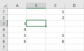
Sub MoveAndCopyCellContents()
    ThisWorkbook.Worksheets("Sheet1").Activate
    ' Move contents from A1:A2 to C1:C2
    Range("A1:A2").Cut Destination:=Range("C1")
    ' Copy contents from A5:A6 to C5:C6
    Range("A5:A6").Copy Destination:=Range("C5")
End Sub

Explanation of the Procedure:

1. Activating the Worksheet:
   The worksheet named « Sheet1 » is activated to ensure all operations are performed on the correct sheet.
2. Moving Cells Using .Cut:

3. Range(« A1:A2 »).Cut Destination:=Range(« C1 »)

• • This line uses the .Cut method to cut (i.e., remove and transfer) the contents from cells A1 to A2.
  • The optional Destination parameter specifies the target range starting at C1.
  • The result is that the contents of A1 and A2 are moved to C1 and C2 respectively.
  • If Destination is not specified, the content is placed in the clipboard, and must then be manually pasted elsewhere.

Copying Cells Using .Copy:

Range(« A5:A6 »).Copy Destination:=Range(« C5 »)

1. • This line uses the .Copy method to duplicate the contents from A5:A6 into C5:C6.
   • As with .Cut, if the destination is not provided, the copied content will be sent to the clipboard for manual pasting.

Visual Outcome:

• Before Running the Procedure:
  The data resides in its original positions: A1:A2 and A5:A6.

• After Running the Procedure:
  • The values from A1:A2 are moved to C1:C2, leaving A1:A2 empty.
  • The values from A5:A6 are copied to C5:C6, so both A5:A6 and C5:C6 now contain the same content.

Why Use This Approach?

Compared to older, more verbose methods involving selection and manual pasting, the .Cut and .Copy methods with the Destination parameter:

• Use fewer lines of code
• Avoid unnecessary selection operations (which can slow down execution)
• Are cleaner and easier to maintain
• Improve code performance and clarity

 

The Cells object in Excel VBA provides a versatile way to access all cells in a worksheet—whether you’re targeting individual cells or entire cell ranges. Instead of using the familiar column-letter and row-number notation (like in the Range object), the Cells object relies solely on numerical indices: the first number represents the row, and the second number represents the column.

This method becomes especially powerful in programmatic contexts, as both the row and column numbers can easily be generated or manipulated using variables.

Example Procedure: Assigning Values Using the Cells Object

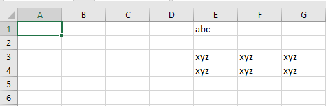
Sub SelectCellsWithCells()
    ThisWorkbook.Worksheets("Sheet1").Activate
    ' Set value in a single cell using Cells
    Cells(1, 5).Value = "abc"
    ' Set value in a range defined by two Cells using the Range object
    Range(Cells(3, 5), Cells(4, 7)).Value = "xyz"
End Sub

Explanation of the Procedure:

1. Activating the Worksheet
   The worksheet « Sheet1 » in the current workbook is activated to ensure that all operations are performed on the correct sheet.
2. Assigning Value to a Single Cell:

3. Cells(1, 5).Value = « abc »

This targets the cell in row 1, column 5, which corresponds to cell E1, and assigns it the value « abc ».

Assigning Value to a Range Defined by Two Cells:

Range(Cells(3, 5), Cells(4, 7)).Value = « xyz »

This defines a rectangular cell block from:

1. • Cells(3, 5) = cell E3
   • to Cells(4, 7) = cell G4

All the cells in this rectangular area (E3:F3:G3, E4:F4:G4) are filled with the value « xyz ».

Why Use the Cells Object?

• It allows for dynamic referencing of cells—perfect when looping through rows and columns.
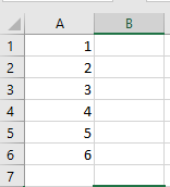
• You can easily integrate row and column variables, e.g.:

• For i = 1 To 10
• Cells(i, 1).Value = i
• Next i
• Compared to Range(« A1 »), Cells(1, 1) is easier to manipulate programmatically—especially in automated or large-scale tasks.

 

Selecting Cells Using the Range Object in VBA

In Excel VBA, the Range object allows you to select both contiguous (connected) and non-contiguous (disconnected) ranges of cells. You define a cell or range by specifying the column letter(s) followed by the row number(s).

Examples of Basic Range Selection (Table 2.1)

VBA Code Example	Description
Range(« A3 »).Select	Selects a single cell A3
Range(« A3:F7 »).Select	Selects a rectangular, contiguous range
Range(« A3, C5, E2 »).Select	Selects multiple, non-contiguous cells
Range(« A8, B2:C4, E2 »).Select	Selects a combination of disconnected individual cells and blocks

These expressions allow flexible selection across the worksheet. However, Range isn’t limited to individual cells or blocks—it can also refer to entire columns or entire rows.

Selecting Full Columns and Rows (Table 2.2)

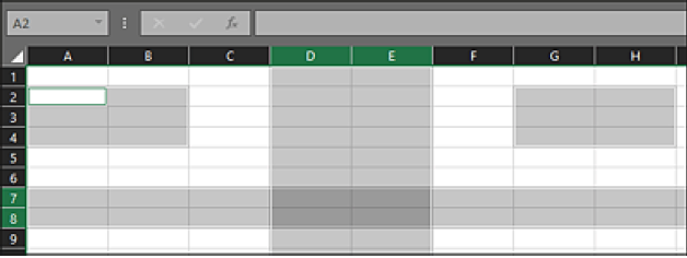
VBA Code Example	Description
Range(« A:A »).Select	Selects the entire column A
Range(« C:E »).Select	Selects three adjacent columns: C, D, E
Range(« B:D, F:F, H:I »).Select	Selects multiple non-adjacent columns
Range(« 3:3 »).Select	Selects the entire row 3
Range(« 3:5 »).Select	Selects rows 3 through 5
Range(« 3:5, 8:9, 12:12 »).Select	Selects multiple non-adjacent rows
Range(« A2:B4, 7:8, D:E, G2:H4 »).Select	Selects a combination of rectangular blocks, entire rows, and entire columns

⚠️ Important: Even though some of these range expressions are long, they must each be written in a single line of code.

In the last example:

Range(« A2:B4, 7:8, D:E, G2:H4 »).Select

A total of four non-contiguous regions are selected:

• Two rectangular areas: A2:B4 and G2:H4
• Two entire rows: 7 and 8
• Two entire columns: D and E

The active cell—the one that appears with a bold outline—is always the top-left cell of the first range listed. So here, the active cell would be A2.

Example Procedure: Selecting Multiple Ranges and Reading Active Cell Address

The following VBA subroutine activates a worksheet and then selects several different cell ranges, each time displaying the address of the active cell using a message box:

Sub SelectCellsWithRange()
    ThisWorkbook.Worksheets("Sheet1").Activate
    ' Select A2 and show active cell address
    Range("A2").Select
    MsgBox ActiveCell.Address
    ' Select a rectangular range and show active cell
    Range("C4:G7").Select
    MsgBox ActiveCell.Address
    ' Select two non-contiguous areas; order affects active cell
    Range("A5, C3:G7").Select
    MsgBox ActiveCell.Address
    ' Same cells as above, but different order
    Range("C3:G7, A5").Select
    MsgBox ActiveCell.Address
    ' Select entire columns C and D
    Range("C:D").Select
    MsgBox ActiveCell.Address
End Sub

Explanation of the Procedure

1. The procedure begins by activating the worksheet named « Sheet1 » in the current workbook.
2. For each selection, the Range(…).Select method highlights the specified cells.
3. The ActiveCell object represents the currently active cell—this is usually the top-left cell in the first range selected.
4. The .Address property is used to return the address of the active cell (e.g., $A$2).

Note: Even if the selected cells are the same, the order in which they are listed in the Range() expression will determine which cell becomes active. For instance:

• Range(« A5, C3:G7 ») → active cell is A5
• Range(« C3:G7, A5 ») → active cell is C3