Étiquette : pratical_excel

As previously explained in  Copying and Moving a Worksheet, to rearrange the order of worksheets, simply drag the worksheet tab to the desired position while holding down the mouse button.A small white sheet icon indicates where the worksheet will be placed.

The second option is to right-click on the worksheet tab and choose Move or Copy.

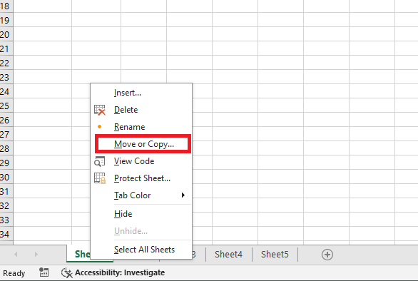
Then, select the desired destination and click the OK button to confirm.

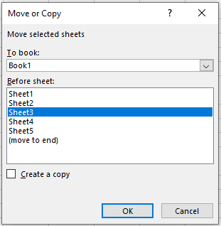
This second option also allows you to move the worksheet to another workbook (note that in this case, you should be careful about maintaining the integrity of cell references between workbooks…).

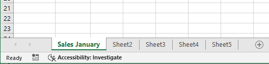
You can improve clarity and navigation in your Excel workbooks by giving each worksheet a name that reflects its content. Excel provides worksheets with generic names such as Sheet1, Sheet2, Sheet3… You can replace these with more descriptive names, such as January Sales, for example.

To rename a worksheet:

• Display the worksheet you want to rename.

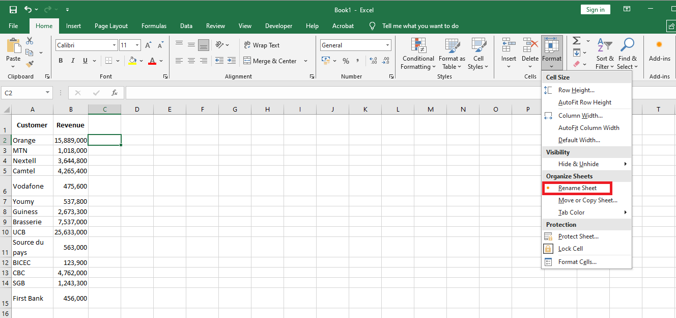
• Click the Home tab,

• Then click Format,

• And finally click Rename Sheet.

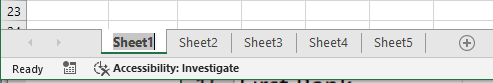
Excel will open the worksheet name for editing and highlight the existing text.

NOTE:
You can also double-click the worksheet tab to rename it.

Please note, however, that although worksheet names can include any combination of letters, numbers, symbols, and spaces, they cannot exceed 31 characters.

NOTE:
If you want to edit the existing name, press the ← or → arrow key to deselect the text, then type the new worksheet name and press Enter. Excel will assign the new name to the worksheet.

You can make it easier to navigate through a workbook by color-coding the worksheet tabs. For example, if your workbook contains sheets related to different projects, you can assign a different tab color to each project. Similarly, you can format tabs for incomplete worksheets with one color and completed worksheets with another. Excel offers 10 standard colors and 60 colors associated with the workbook’s current theme.

You can also apply a custom color if none of the standard or theme colors meet your needs. To change the worksheet tab color, click the tab of the worksheet you want to format.

Then, click the Home tab, click Format, and finally click Tab Color.

Excel displays the tab color palette. Click the color you want to apply to the current tab.

The tab color appears faintly when the tab is selected, but it shows more vividly when another tab is selected.

NOTE:
To apply a custom color, click More Colors, then use the Colors dialog box to choose your desired color.

NOTE:
You can also right-click the tab, click Tab Color, and then click the color you want to apply.

Excel allows you to insert hyperlinks into cells. There are many things you can do with hyperlinks in Excel (such as linking to an external website, linking to another sheet/workbook, linking to a folder, linking to an email address, etc.).

How to Insert Hyperlinks in Excel
There are several ways to create hyperlinks in Excel. You can:
■ Type the URL manually (or copy and paste it)
■ Use the HYPERLINK function
■ Use the Insert Hyperlink dialog box

Type the URL Manually
When you manually enter a URL in an Excel cell or copy and paste it into the cell, Excel automatically converts it into a hyperlink.
Here are the steps to turn a plain URL into a hyperlink:

• Select a cell where you want to insert the hyperlink

• Press F2 to enter edit mode (or double-click the cell)

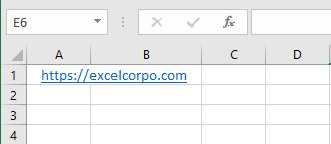
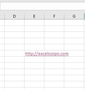
• Type the URL and press Enter. For example, if I type the URL – https://excelcorpo.com into a cell and press Enter, it will create a hyperlink to that address.

NOTE
Please note that you must include http or https for URLs that do not have www. If the URL starts with www, Excel will still create the hyperlink even if you do not add http/https.

When you copy a URL (document/file) and paste it into an Excel cell, it will automatically be hyperlinked.

Insert a Link Using the Dialog Box
If you want the cell’s display text to be something other than the URL and still link it to a specific web address, you can use Excel’s Insert Hyperlink option.

Below are the steps to insert a hyperlink into a cell using the Insert Hyperlink dialog box:

Select the cell where you want to insert the hyperlink

Type the text you want to display as the hyperlink. For example: « ExcelCorpo Company »

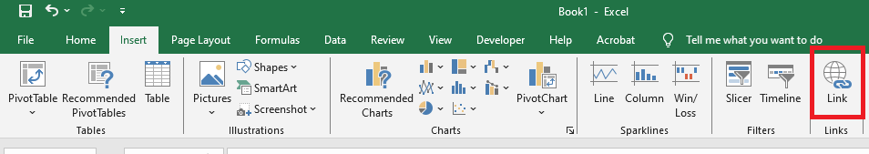
Click the Insert tab on the ribbon

Click the Links button. This will open the Insert Hyperlink dialog box (you can also use the keyboard shortcut Ctrl + K)

In the Insert Hyperlink dialog box, enter the URL into the Address field

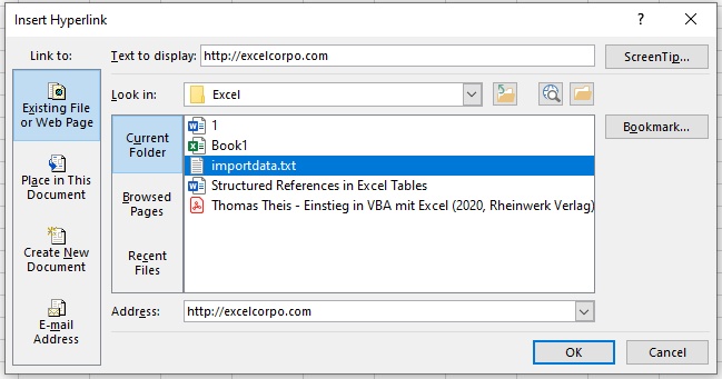
Click the OK button

This will insert the hyperlink into the cell while keeping the display text unchanged.

NOTE:
There are many more things you can do with the Insert Hyperlink dialog box (such as creating a hyperlink to another worksheet in the same workbook, linking to a document/folder, linking to an email address, etc.).

Insert Using the HYPERLINK Function
Another way to insert a link in Excel is by using the HYPERLINK function. In general, the HYPERLINK function creates a shortcut that opens another location in the current document or opens a document stored on a network server, intranet, or the Internet.
When you click a cell that contains the HYPERLINK function, Excel opens the location indicated or launches the document you specified. Its syntax is:

HYPERLINK(link_location, [friendly_name])
with:
■ link_location: This can be the URL of a webpage, the path to a folder or file on your hard drive, or a reference within a document (such as a specific cell or named range in a worksheet or Excel workbook).
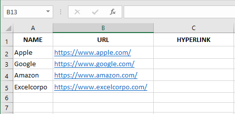
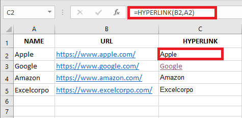
■ [friendly_name]: This is an optional argument. It’s the text you want to display in the cell that contains the hyperlink. If you omit this argument, Excel will use the link_location text as the display text.

Below is an example where I have company names in one column and their website URLs in another.

The HYPERLINK function shown below generates a result where the display text is the company name and it links to the company’s website.

So far, we’ve seen how to create hyperlinks to websites. However, you can also create hyperlinks to worksheets within the same workbook, other workbooks, or files and folders on your hard drive.

Create a Hyperlink to a Worksheet in the Same Workbook
Here are the steps to create a hyperlink to Sheet2 within the same workbook:

Select the cell where you want to insert the hyperlink

Type the text you want to display as the hyperlink. In this example, I used the text « Link to Sheet2 »

Click the Insert tab

Click the Links button. This will open the Insert Hyperlink dialog box (you can also use the keyboard shortcut Ctrl + K)

In the Insert Hyperlink dialog box, select Place in This Document from the left pane

Enter the cell you want to hyperlink to (I’ll use A1 as the default)

Select the worksheet you want to link to (Sheet2 in this case)

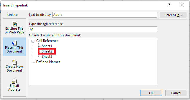
Click OK

NOTE:
You can also use the same method to create a hyperlink to any cell within the same workbook. For example, if you want to link to a distant cell (say K100), you can do so by entering that cell reference in Step 6 and selecting the appropriate worksheet in Step 7.

You can also use the same method to create a hyperlink to a named range. If you have named ranges in the workbook, they will be listed under the Defined Names category in the Insert Hyperlink dialog box.
In addition to the dialog box, Excel also provides a function that allows you to create hyperlinks.
So instead of using the dialog box, you can use the HYPERLINK formula to create a link to a cell in another worksheet. The following formula does exactly that:

Here’s how this formula works:
■ "#" tells the formula to refer to the same workbook
■ "Sheet2!A1" specifies the cell to be linked in the same workbook
■ "Link to Sheet2" is the display text in the cell

Create a Hyperlink to a File (in the Same Folder or Different Folders)

You can also use the same method to create hyperlinks to other Excel files located in the same folder or in different folders. For example, if you want to open a file named Test.xlsx located in the same folder as your current file, you can follow these steps:

Select the cell where you want the hyperlink

Click the Insert tab

Click the Links button. This opens the Insert Hyperlink dialog box (you can also use the shortcut Ctrl + K)

In the Insert Hyperlink dialog box, select Existing File or Web Page in the left pane

Choose Current Folder from the « Look in » options

Select the file you want to link to. Note that you can link to any type of file (Excel or non-Excel files)

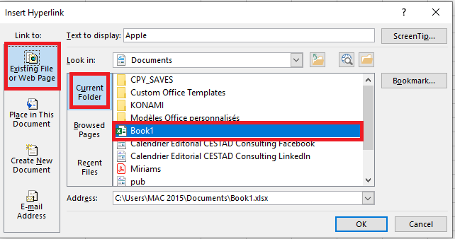
(Optional) Replace the display text if you wish

Click OK

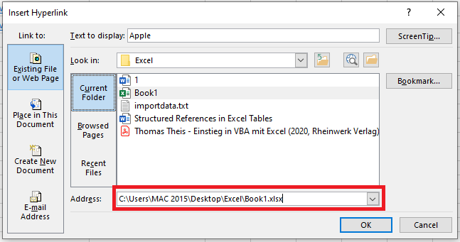
If the file is not in the same folder, you can browse for the file and select it. To browse, click the folder icon in the Insert Hyperlink dialog box.
You can also do this using the HYPERLINK function. The formula below creates a hyperlink to a file in the same folder as the current file:

If the file is in a different folder, copy the full file path and use it as the link_location.

Create a Hyperlink to a Folder

Here are the steps to create a hyperlink to a folder:

Copy the path of the folder you want to link to

Select the cell where you want the hyperlink

Click the Insert tab

Click the Links button to open the Insert Hyperlink dialog box (or use Ctrl + K)

In the Insert Hyperlink dialog box, paste the folder path

Click OK

You can also use the HYPERLINK function to create a hyperlink that points to a folder. For example, the formula below will create a hyperlink to a folder named data analysis. When you click the cell, the folder will open:

To use this formula, replace the folder path with the one you want to link to.

Create a Hyperlink to an Email Address

You can also create hyperlinks that open your default email client (such as Outlook) with the recipient’s address and subject line pre-filled.
Here are the steps to create an email hyperlink:

Select the cell where you want the hyperlink

Click the Insert tab

Click the Links button to open the Insert Hyperlink dialog box (or press Ctrl + K)

In the Insert Hyperlink dialog box, click Email Address under the « Link to » options

Enter the email address and subject line

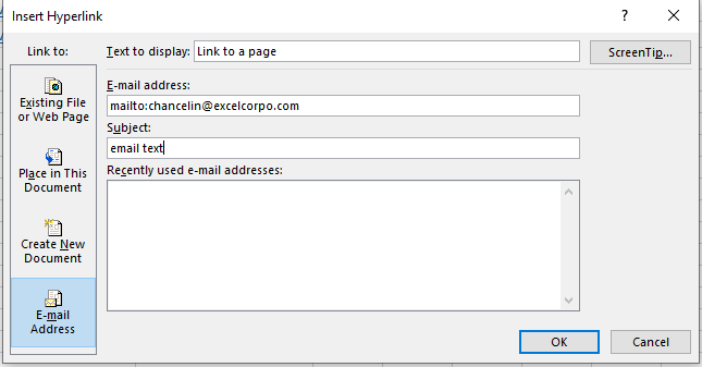
(Optional) Type the display text you want in the cell

Click OK

Now, when you click the cell containing the hyperlink, it will open your default email client with the recipient and subject line already filled in.
You can also do this using the HYPERLINK function. The formula below opens the default mail client and pre-fills the recipient’s address:

The Go To Command

When editing a worksheet, the Go To command and the Go To Special command can be very useful. For instance, if you know the reference of the cell or range you want to navigate to, using the Go To command is quicker and more efficient. Once used, a list of previously visited cells and ranges appears in the list box. You can easily return to those locations by clicking the references and then clicking OK, or simply by double-clicking the reference.

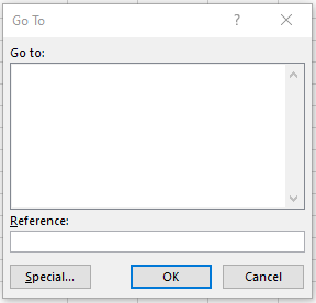
Additionally, after using the Go To command, the Reference box at the bottom of the dialog displays your previous location. To return to it, simply press Enter or click OK. This feature allows you to switch between two locations by pressing F5 and Enter.

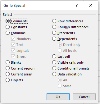
The Special… button in the Go To dialog provides a mechanism to select specific ranges based on cell content. When you click this button, the Go To Special dialog appears, as shown in Figure .

Many of these options are helpful when reviewing or auditing a worksheet. For example, you might want to select all formulas that return error values. Simply select Formulas and check the Errors box, making sure to uncheck the other formula types.

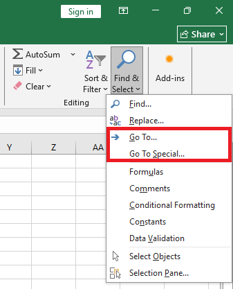
How to Open the Go To Dialog

You can open the Go To dialog in three different ways:

Using the Excel shortcut: Press Ctrl + G / The Go To dialog opens / Click the Special button or press Alt + S / The Go To Special dialog opens.

Using the function key: Press F5 / The Go To dialog opens / Click the Special button or press Alt + S / The Go To Special dialog opens.

Using the Ribbon: Go to the Home tab / In the Editing section, from the drop-down menu, click Find & Select / Choose Go To or Go To Special (both options are available).

Options in the Go To Special Dialog:

• Comments – Cells that contain comments.
• Constants – Cells that contain constant data (text, numbers, or dates), as opposed to formulas. Check or uncheck the boxes for numbers, text, or formulas to specify what to include in the selection.
• Formulas – Cells that contain formulas (i.e., start with « = ») and not constants. Check or uncheck boxes for numbers, text, logical values, and errors to specify what to include.
• Blanks – Cells that contain neither data nor formatting. Excel automatically ignores each blank cell below and to the right of the last cell containing data.
• Current Region – The active cell and all adjacent cells bounded by blank rows and columns.
• Current Array – Selects all cells in an array formula.
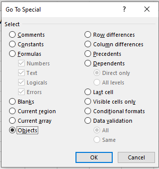
• Objects – All objects in the worksheet, including charts, text boxes, and shapes.
• Row Differences – Selects cells that differ from the comparison cell in each row. The comparison cell is in the same column as the active cell.
• Column Differences – Similar to Row Differences but works by column.
• Precedents – Cells that the active cell refers to. Choose Direct only (default) or All levels to include indirect references.
• Dependents – Cells that refer to the active cell. Choose Direct only (default) or All levels to include indirect references.
• Last Cell – The last « used » cell in the active worksheet, including formatting. This is automatically updated—no need to close the workbook.
• Visible Cells Only – Selects only cells that are visible (not hidden). Useful for copying only filtered rows from a table.
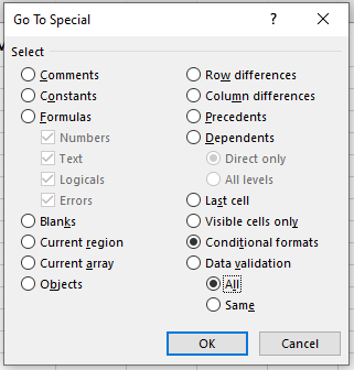
• Conditional Formats – Cells with conditional formatting applied. Choose All (default) to select all such cells or Same to select only those with the same formatting as the active cell.
• Data Validation – Cells with data validation rules. Choose All (default) to select all such cells or Same to select only those with the same validation rule as the active cell.

Using the Go To Special Command

The Go To Special dialog box in Excel contains many options for selecting cells based on the type of content they contain.

Example 1: Using the Comments Option
Select any cell within a range → Press Ctrl + G or the F5 key to open the Go To dialog box → Click the Special… button to open the Go To Special dialog → Choose the Comments radio button → Click OK or press Enter to select all cells that contain a comment.

Example 2: Using the Constants Option
Select any cell within a range → Press Ctrl + G or F5 to open the Go To dialog → Click Special… to open the Go To Special dialog → Choose the Constants radio button.
By default, Excel checks Numbers, Text, Logicals, and Errors → Click OK or press Enter to select all cells that contain constant values (numbers, text, logicals, or errors), but not formulas.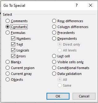

Example 3: Using the Formulas Option
Select any cell within a range → Press Ctrl + G or F5 to open the Go To dialog → Click Special… to open the Go To Special dialog → Choose the Formulas radio button.
By default, Excel checks Numbers, Text, Logicals, and Errors → Click OK or press Enter to select all cells containing formulas (i.e., starting with an equals sign =).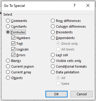

Example 4: Using the Errors Option
If you select the Constants radio button and only check the Errors checkbox, Excel will select all error values that are not in formulas.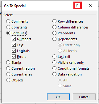

Similarly, if you select the Formulas radio button and check Errors, Excel will select all cells containing formulas that return an error.

Example 5: Using the Blanks Option

Select any cell in a range → Press Ctrl + G or F5 to open the Go To dialog box → Click Special… to open the Go To Special dialog → Choose the Blanks radio button → Click OK or press Enter to select all blank cells.
After selecting the blank cells, you can apply fill color or enter a value (e.g., zero ‘0’). For instance, type 0 in one cell, then press Ctrl + Enter to fill all selected blank cells with 0.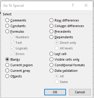

Example 6: Using the Objects Option

Select any cell in a range → Press Ctrl + G or F5 to open the Go To dialog box → Click Special… to open the Go To Special dialog → Choose the Objects radio button → Click OK or press Enter to select all objects, including text boxes.

Example 7: Using the Conditional Formats Option

Select any cell in a range → Press Ctrl + G or F5 to open the Go To dialog box → Click Special… to open the Go To Special dialog → Choose the Conditional Formats radio button → Press Enter to select only the cells that have conditional formatting applied.

Create, Use, Edit, and Delete Named Ranges

Names are a convenient identity. Imagine how difficult it would be to refer to someone if they had no name! Excel offers a similar convenience by allowing you to define named ranges.

What Is a Named Range?

In Excel, a single cell or a range of cells can be assigned a name to simplify their use. Named ranges can be used directly in formulas or for quickly selecting that range.

You can name:

• A range of cells

• A formula

• A constant

• A table

Benefits of Creating Named Ranges

The main advantage of using named ranges is the simplicity and clarity they provide.

• You don’t need to memorize or look up cell references when writing formulas—you can use the named range instead.

• Using named ranges reduces typing errors, since names can be selected from a list.

• They are especially helpful in formulas, as Excel suggests named ranges when typing the first few letters.

• Named ranges make formulas portable, allowing them to be reused across sheets or workbooks.

• A dynamic named range can automatically expand or shrink as data is added or removed—no need to manually update formulas.

• Named ranges are useful in data validation, such as creating drop-down menus.

• You can quickly create hyperlinks to named ranges for easier navigation.

• Named ranges make navigation and direction within a workbook easier—click a name in the Name Box to jump to that range.

• Despite all these benefits, creating a named range is simple and fast.

Naming Rules for Named Ranges

When creating named ranges in Excel, the following rules must be observed:

• A name must be less than 255 characters.

• A name cannot contain spaces or punctuation characters (except as noted below).

• The first character must be a letter, an underscore (_), or a backslash (\).

• A name may include a question mark (?), but it cannot be the first character.

• Names are not case-sensitive. For example, sales, Sales, and SALES are treated as the same name.

• A name must not resemble a cell reference (e.g., A1, A$1).

• A name can consist of a single letter but must not be R, r, C, or c, since « R » and « C » are reserved as shortcuts for row and column selection.

How to Create Named Ranges

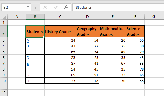
There are two main methods for creating named ranges in Excel. We’ll demonstrate both using the example of assigning two named ranges—one for history grades and another for geography grades.

Method 1 – Creating a Named Range Using the Name Box

This method is simple:
Select the range → Type the desired name in the Name Box → Press Enter.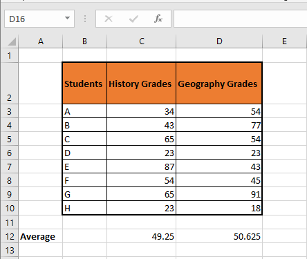

To name the range for History Grades, follow these steps:

Select cells C3:C10 (history scores)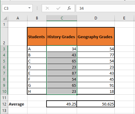

Click in the Name Box

Type History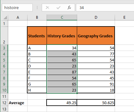

Press Enter

Method 2 – Creating a Named Range Using the “Define Name” Option

Named ranges can also be created via the Define Name button in the Formulas tab.

Select the range you want to name (in this case, D3:D10 for geography scores)

Go to the Formulas tab and click Define Name

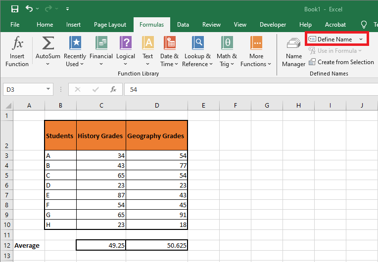
In the New Name window, enter the desired name

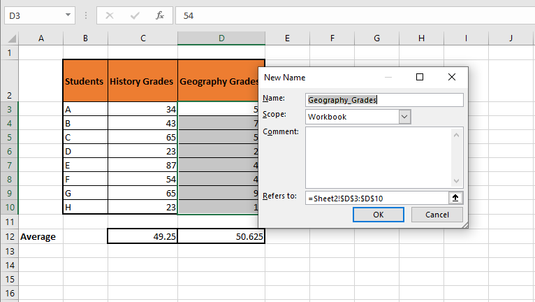
Click OK to confirm

How to Edit Named Ranges in Excel

Suppose you missed a cell in the range or want to rename the named range—you’ll need to edit it.

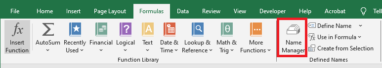
This is done via the Name Manager, found under Formulas > Name Manager, or by pressing Ctrl + F3.

In the Name Manager, you will see a list of named ranges and their details.

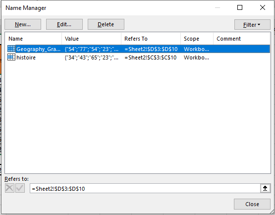
To modify a named range:

Double-click it, or

Select it and click the Edit… button

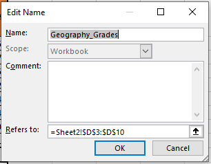
This opens the Edit Name window, where you can change the name or the reference range.
Click OK, then Close the Name Manager when done.

How to Delete Named Ranges

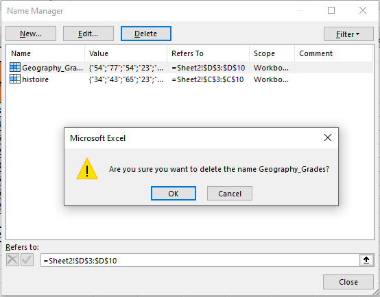
You can also use the Name Manager to delete named ranges:

Select the name to delete

Click the Delete button

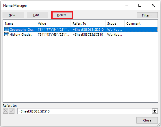
A confirmation message will appear asking if you really want to delete it—click OK.

Tip:
The Name Manager also includes a Filter button that lets you display only relevant named ranges. This is especially helpful when dealing with a large number of names.

Create Names from Cell Text

When dealing with structured datasets—whether in columns with headers at the top or rows with labels on the left—you can quickly name multiple ranges using Excel’s Create from Selection feature. This tool assigns names to ranges based on adjacent header cells.

Let’s consider a dataset showing students’ scores in various subjects, laid out in columns. We can use « Create from Selection » as follows:

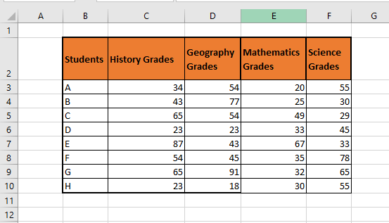
Select the entire range including the headers. In our case, we’ll select columns C, D, E, and F to name each column range based on its header.

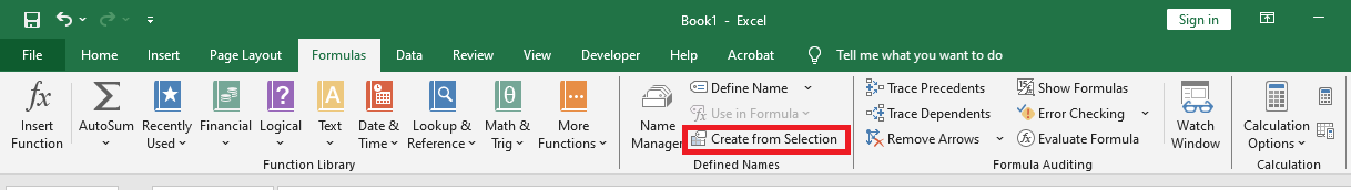
Go to the Formulas tab and click Create from Selection, or press the shortcut Ctrl + Shift + F3.

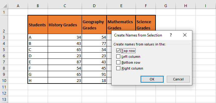
Based on the layout, choose the location of the headers. In our example, select Top row, since headers like « History Grades », « Geography Grades », « Math Grades », and « Science Grades » are in the top row.

Click OK.

Excel will create named ranges based on the headers. In the Name Box, you’ll now see four named ranges corresponding to each subject column.

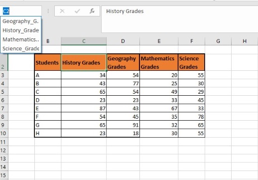
Note: Spaces in header names are automatically replaced with underscores in named ranges.

Named Ranges with Hyperlinks

If you thought named ranges made navigating a workbook easier, just wait until you combine them with hyperlinks. Named ranges simplify hyperlink creation by pointing directly to structured, predefined data areas.

Let’s see how it works:

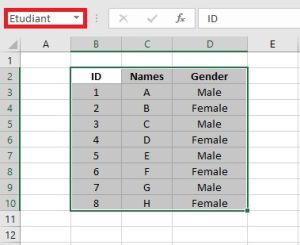
Suppose we have a named range called Students in Sheet2.

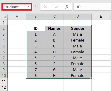
Now, we’ll create a hyperlink from Sheet1 that jumps to this named range in Sheet2.

Select the Students range in Sheet2 (e.g., B3:B10)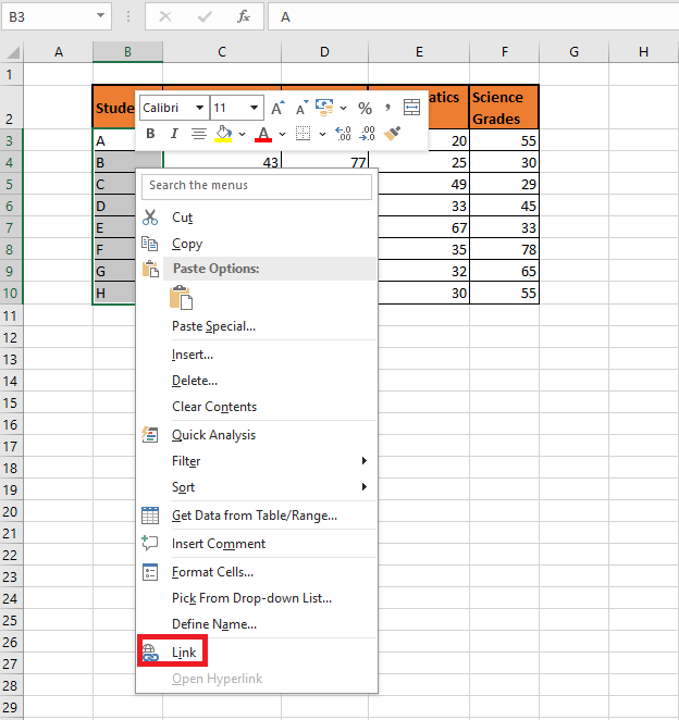

Right-click the selection and choose Link. The Insert Hyperlink window will appear.
 

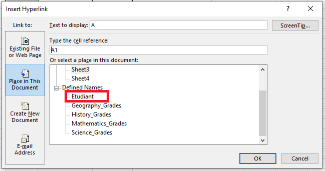
Under Defined Names, select Students, which we previously created.

Click OK.

You’ve now created a hyperlink pointing to the Students range in Sheet2. Clicking it from Sheet1 will instantly navigate you to that range.

Creating a Named Range for a Constant

The Name Manager can also be used to define named constants—fixed values that don’t refer to a cell but can be reused in formulas.

In this example, we’ll define a constant to calculate the percentage of total marks for 5 students. Assume each subject is graded out of 100, with 4 subjects total, making 400 the maximum score.

Open the Name Manager and click New.

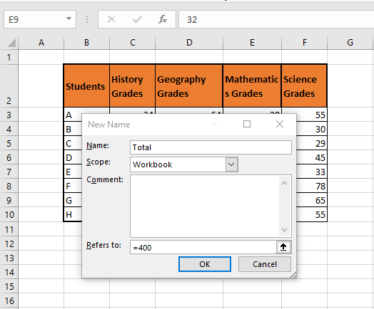
Define « total » as the name, and set its value to 400.

Now, in formulas, you can simply use total instead of typing 400 repeatedly.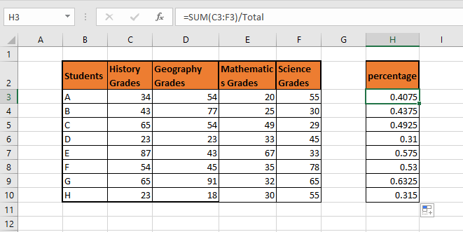

Formulas Using Named Ranges

Following the example above, what if we named the entire formula instead of just the constant? This would let us calculate student percentages with a single named formula.

Open the Name Manager again and click New.

Define the name as « Percentage ».

In the Refers to field, enter:

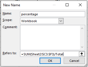
Here, C3:F3 is the range of marks to be summed.
The column references are made absolute ($C:$F), while row references remain relative so that the formula can be filled down for each student.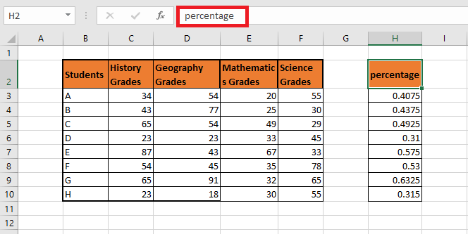

Now, by simply entering =Percentage, you can apply the full formula across multiple rows.

Named Ranges for Data Validation

Named ranges make Excel’s Data Validation feature a breeze. You can create a drop-down list from a named range.

This approach offers several advantages: you simply reference the named range in the Data Validation window instead of manually entering cell ranges. It also provides better visibility and clarity when managing the list source.

Let’s walk through an example.

Suppose we have a list of products, along with their prices and available discounts. Our goal is to calculate the final discounted price per product after selecting a discount from a drop-down list in column D.

We’ll create a drop-down menu using the named range "Discount" (G3:G6).

Select the cells where you want to apply the drop-down list (D3:D9).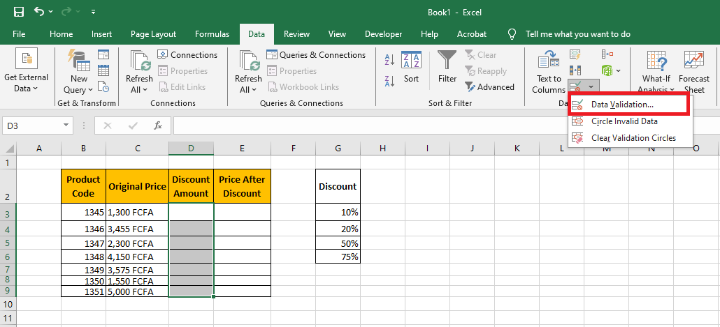

Go to the Data tab → Data Tools section → Click Data Validation → Choose Data Validation from the dropdown.

In the Data Validation window:

Under Allow, choose List.

Under Source, enter the named range: =Discount.

Click OK.

This will create drop-down menus in cells D3 through D9 populated with values from the "Discount" named range.

Now, users can simply select applicable discounts and proceed to calculate the final discounted prices.

Scope of a Named Range

If you open the Name Manager, you’ll notice each named range has a scope (e.g., Sheet1, Sheet2, Workbook).

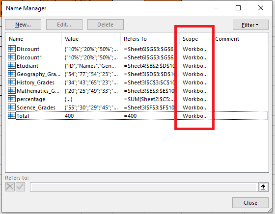
The scope defines where the name is recognized and accessible.

Types of Scope:

• Worksheet-Level Scope
  A locally scoped name is recognized only on the worksheet where it was created.
  This means you can have multiple worksheets with the same named range, each specific to its own sheet.

For example, in a workbook with one sheet per month, each sheet could have a named range called "Expenses".

Pro tip:
Named ranges created via the Name Box have workbook-level scope by default.
To create a local name, prefix it with the worksheet name followed by an exclamation point:

• Workbook-Level Scope
  A globally scoped name can be used throughout the entire workbook.
  Such names must be unique within the workbook.

Example: You can define a global constant named "pi" with the value 3.14 and use it in formulas across all worksheets.

Navigate a Worksheet Using the Keyboard

You can use several keyboard shortcuts to move around a worksheet efficiently—especially useful during data entry, when keeping your hands on the keyboard saves time.