Votre panier est actuellement vide !
Étiquette : pratical_excel
Inspect a Workbook for Compatibility Issues in Excel
You can check for compatibility between different versions of your Microsoft Office files to see whether the features in a file are supported in earlier versions of Office using the Compatibility Checker.
To check compatibility with an earlier version of Office:
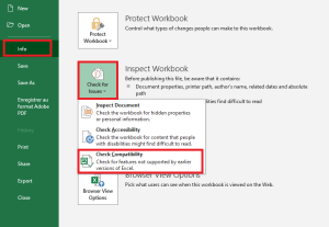
- Click the File tab, then select Info.
- Click Check for Issues, then Check Compatibility.
Selecting Check Compatibility when saving documents in the Compatibility Checker window prompts the Office application to automatically verify compatibility issues when saving your file in an earlier version format.
Important:
■ Before saving an Excel 2007 or later workbook in an earlier file format, you must fix any issues that could result in significant loss of functionality in order to prevent permanent data loss or incorrect behavior. Excel’s Compatibility Checker can help identify potential problems.
■ Issues that cause minor fidelity loss may or may not be addressed before proceeding with the file save. These do not result in data or feature loss, but the file may look or behave differently when opened in an earlier version of Microsoft Excel.The Compatibility Checker automatically launches when you attempt to save a file in the Excel 97-2003
.xlsformat. If potential issues do not concern you, you can disable compatibility checking.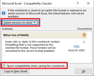
If you have upgraded to a new version of Excel and realize you will be sharing workbooks with people who haven’t yet upgraded, running the Compatibility Checker helps you identify features or content that may not be supported in older versions, allowing you to address these issues before sharing your workbook. Save the file in
.xlsformat and review any issues detected by the Compatibility Checker.Proceed as follows:
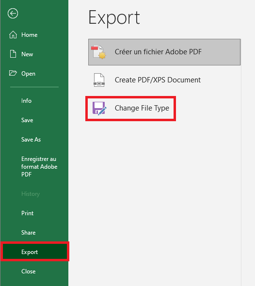
- Click File > Export > Change File Type.
- Under Workbook File Types, double-click Excel 97-2003 Workbook (*.xls).
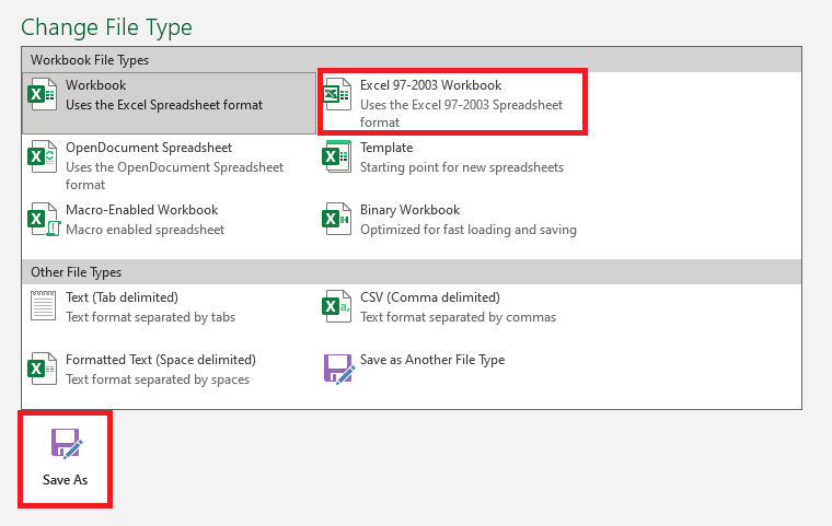
- In the pop-up Save As window, choose a folder location for the workbook.
- In the File Name box, type a new file name (or use the existing one).
- Click Save.
- If the Compatibility Checker appears, review the compatibility issues that were found.
Figure 1.5.8-c: Accessibility Issues
The Find link lets you jump to the relevant location in your worksheet, and the Help link provides more information on the issue and possible solutions.
Notes:
■ In your newer version of Excel, any file opened in.xlsformat opens in Compatibility Mode. Continue working in this mode if you intend to send the workbook repeatedly to people using an older version of Excel.
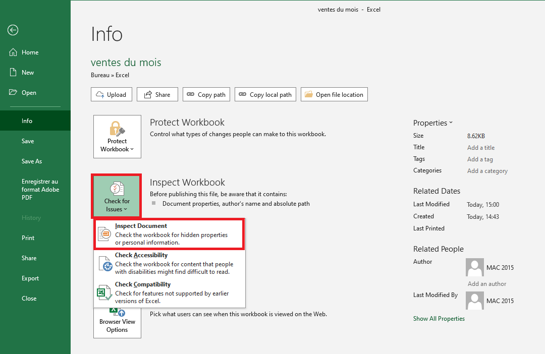
■ When backward compatibility is no longer needed, click File > Info > Convert to upgrade the workbook to the current file format and take advantage of new Excel features.Inspecting a Workbook for Hidden Properties or Personal Information in Excel
Excel offers several features that help ensure your workbooks appear and function as intended before distributing them to others. It provides many options to help you prepare a workbook for sharing.
Inspect a Workbook
Check the workbook for hidden information such as personal details, custom XML data, and other concealed or embedded information. This hidden data may reveal details about your organization or the workbook itself that you might not want to share publicly. You can remove this hidden information before sharing the workbook with others.
-
Click the File tab.
-
Click Info.
-
Click Check for Issues.
-
Click Inspect Document.

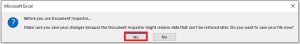
- Click Yes.
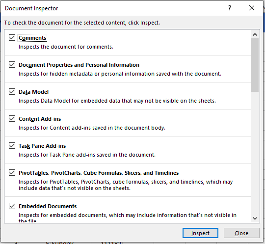
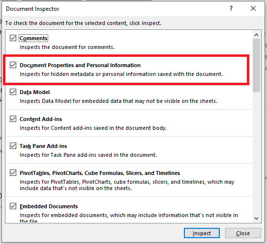
There are various elements you can check in your workbook. Browse through the list and identify the hidden content you want to inspect.
-
Check the boxes for the items you wish to inspect.
-
Click Inspect.
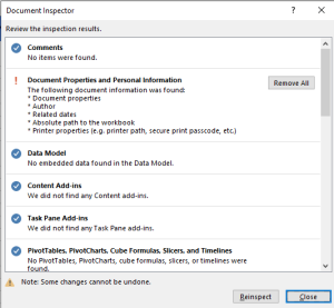
-
Click Remove All next to the items you want to delete.
-
Click Close.
 Z
ZThe hidden data is now removed from the workbook and will not be visible to others.
Protect Your Workbook
By default, anyone with access to your workbook can open, copy, and edit its contents unless you protect it. There are several ways to protect a workbook, depending on your needs.
To protect your workbook:
-
Click the File tab to access Backstage view.
-
In the Info pane, click the Protect Workbook command.
-
From the drop-down menu, choose the option that best suits your needs.
In our example, we’ll select Mark as Final.
Marking your workbook as final is a good way to discourage others from editing it, while other options provide even more control if necessary.
-
A dialog box will appear prompting you to save. Click OK.

-
Another dialog box will appear. Click OK.
-
The workbook will now be marked as final.

Note: Marking a workbook as final does not prevent others from editing it. If you want to prevent modifications, you can use the Restrict Access option instead.
-
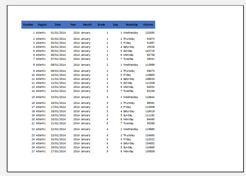
Displaying Repeated Row and Column Headers on Multipage Worksheets in Excel
If you often need to print large and complex Excel worksheets, then you’ve likely encountered this issue. While you can easily scroll through the document from top to bottom without losing sight of the column headers because the header row is frozen, when printing the document, the top row is only printed on the first page.
If you’re tired of flipping through printed pages to find out what kind of data each column or row contains, this section provides the solution.
Repeat Excel Header Rows on Every Page
Your Excel document turns out to be long and you need to print it. You go to Print Preview and notice that only the first page has column headers at the top. You can specify the page setup options to repeat the top row on every printed page.
- Open the worksheet you’re going to print.
- Go to the Page Layout tab.
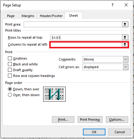
- Click Print Titles in the Page Setup group.
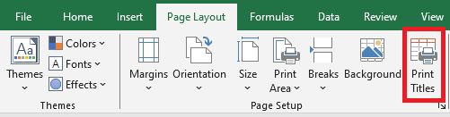
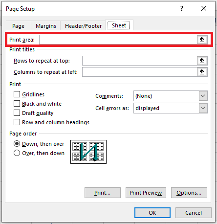
- Make sure you are on the Sheet tab in the Page Setup dialog box.
- Look for the Rows to repeat at top field under the Print Titles section.
- Click the Collapse Dialog icon next to the “Rows to repeat at top” field.
The Page Setup dialog box collapses and returns you to the worksheet. You’ll notice the cursor turns into a black arrow, which makes it easy to select an entire row with a single click.

- Select one or more rows that you want to print at the top of every page.
To select multiple rows, click the first row, hold the mouse button, and drag to the last row you want to include.
- Press Enter or click the Collapse Dialog button again to return to the Page Setup dialog.
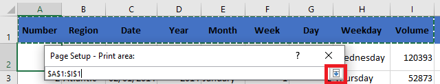
Now, your selection appears in the Rows to repeat at top field.
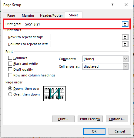
You can skip steps 6 to 8 and manually enter the range using the keyboard. Be careful to use absolute references (with the dollar sign
$). For example, to repeat the first row on every page, type:$1:$1.- Click Print Preview to view the result.
 Repeat Header Columns on Every Printed Page
When your worksheet is too wide, the header column appears only on the left side of the first printed page. To make your document more readable, follow the steps below to print the row header column on the left side of every page:
- Open the worksheet you want to print.
- Follow steps 2 to 4 from the previous section (Repeat header rows).
- Click the Collapse Dialog button next to the Columns to repeat at left field.
- Select one or more columns that you want to repeat on every printed page.
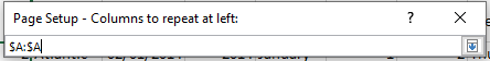
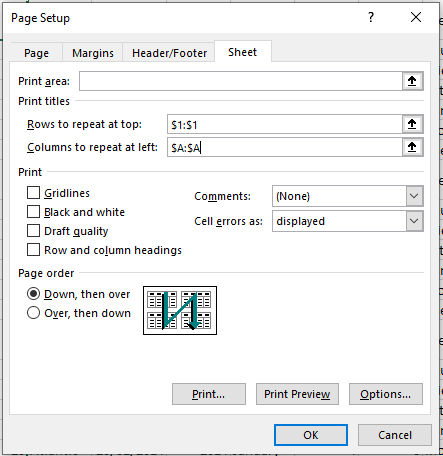
- Press Enter or click the Collapse Dialog button again to confirm that the selected range appears in the Columns to repeat at left field.
- Click Print Preview in the Page Setup dialog box to preview your document before printing.

Now, you won’t have to flip pages to figure out the meaning of each row’s values.
Print Row Numbers and Column Letters
Excel normally refers to worksheet columns by letters (A, B, C) and rows by numbers (1, 2, 3). These letters and numbers are called row and column headers. Unlike row and column titles, which are only printed on the first page by default, headers are not printed at all.
If you want to see these letters and numbers on your printed pages, follow these steps:
- Open the worksheet you want to print with row and column headers.
- Go to the Sheet Options group on the Page Layout tab.
- Check the box Print under Headings.
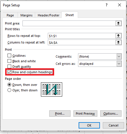
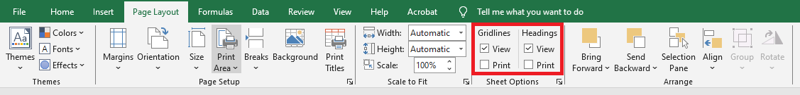 If the Page Setup dialog box is already open on the Sheet tab, simply check the box Row and column headings under the Print section.
This will make the row and column headers visible on every printed page.
- Open the Print Preview pane (File > Print or Ctrl + F2) to verify the changes.
The Print Titles command can really simplify your work. Printing row and column headers on each page makes it easier to understand the information in your document. You won’t get lost in the printouts if every page includes the appropriate row and column titles. Try it — and you’ll appreciate the difference!
Setting Print Scaling in Excel
Usually, you’ll often need to make small adjustments from the Print pane to perfectly fit your workbook’s contents onto a printed page. The Print pane includes several tools to help you adjust and scale your content, such as scaling, page margins, and sheet orientation.
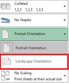
To change the page orientation, Excel offers two options: Landscape and Portrait. Landscape orients the page horizontally, while Portrait orients it vertically. In our example, we will set the page orientation to Landscape.
- Go to the Print pane.
- Select the desired orientation from the Page Orientation drop-down menu. In our example, we will select Landscape Orientation.
- The new page orientation will be displayed in the Preview pane.

Adjusting Content Before Printing
If part of your content is cut off by the printer, you can use scaling to automatically fit your workbook to the page.- Go to the Print pane. In our example, we can see in the Preview pane that part of the content will be cut off when printed.
- Select the desired option from the Scaling drop-down menu. In our example, we’ll choose Fit All Columns on One Page.
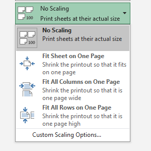
- The worksheet will be condensed to fit on a single page.
Keep in mind that worksheets become harder to read as they are reduced in size, so you may want to avoid this option when printing a sheet with a lot of data.
- Click the Page Break Preview command to switch to Page Break mode.

- The dotted blue vertical and horizontal lines indicate page breaks. Click and drag one of these lines to adjust the page break.
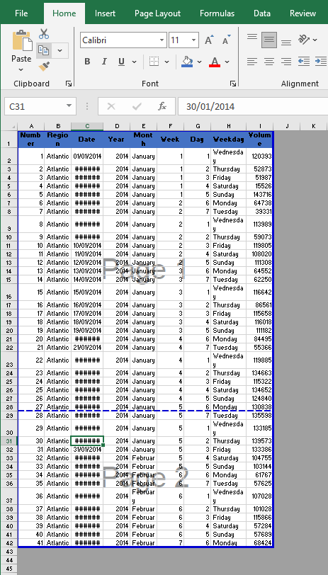
- In our example, we set the horizontal page break between rows 21 and 22.
- In our example, all pages now display the same number of rows because of the page break adjustment.

Adjust margins in the Preview pane
A margin is the space between your content and the edge of the page. Sometimes, you may need to adjust the margins to make your data more readable. You can change the page margins from the Print pane.
- Go to the Print pane.
- Select the desired margin size from the Page Margins drop-down menu. In our example, we’ll select Narrow.
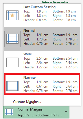
- The new page margins will be displayed in the Preview pane.
You can manually adjust the margins by clicking the Show Margins button in the lower-right corner and then dragging the margin markers in the Preview pane.

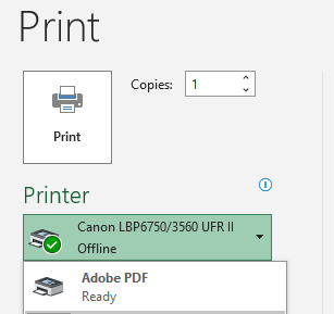
Print All or Part of a Workbook in Excel
You may sometimes want to print a workbook to view and share your data offline. Once you’ve chosen your page layout settings, it’s easy to preview and print a workbook from Excel using the Print pane.
To access the Print pane:
- Click the File tab. The Backstage view will appear.
- Select Print. The Print pane will appear.
 Click the buttons in the interactive figure below to learn more about using the Print pane.
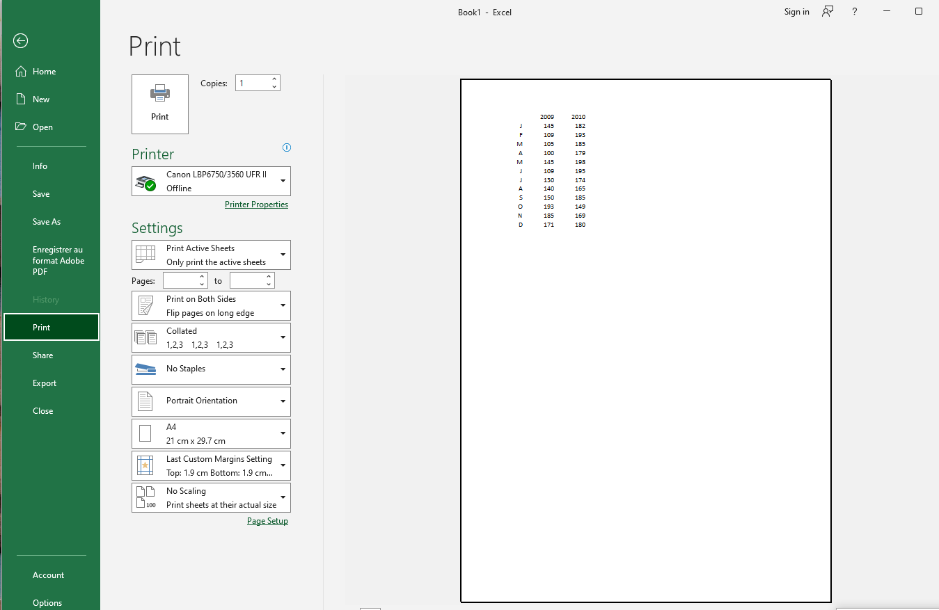
To print a workbook:
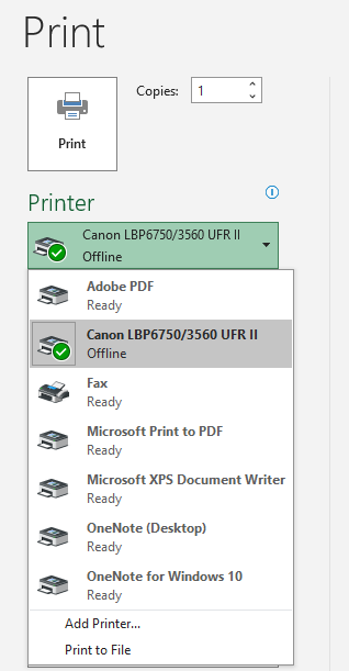
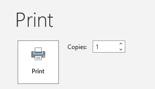
- Go to the Print pane, then select the printer you want to use.
- Enter the number of copies you want to print.

- Select additional settings if needed (see interactive figure above).
- Click Print.
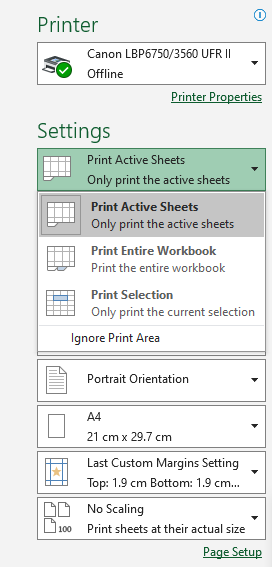
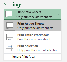
Before printing an Excel workbook, it’s important to decide exactly what information you want to print. For instance, if your workbook contains multiple worksheets, you’ll need to decide whether to print the entire workbook or only the active sheets. You may also wish to print only a specific selection of content from your workbook.
To print active sheets:
Worksheets are considered active when they are selected.- Select the worksheet you want to print. To print multiple worksheets, click the first sheet, then hold down the Ctrl key on your keyboard and click the other sheets you want to select.
- Go to the Print pane.
- In the Print Range dropdown, select Print Active Sheets.
- Click the Print button.
To print the entire workbook:
- Go to the Print pane.
- In the Print Range dropdown, select Print Entire Workbook.
- Click the Print button.
To print a selection:
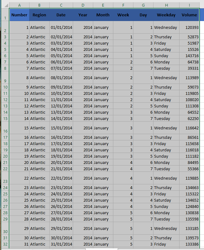
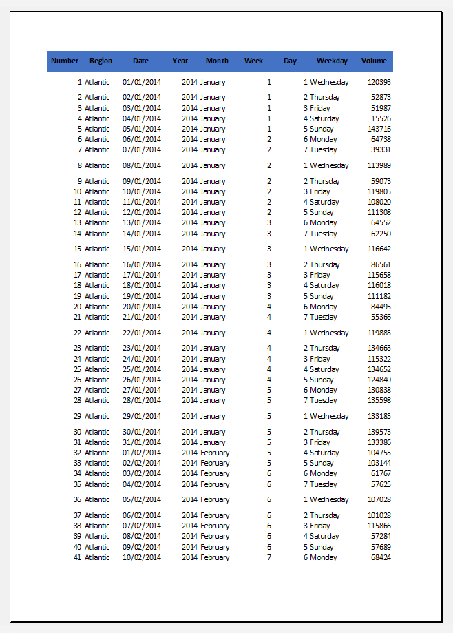
In this example, we will print the first 40 rows of the worksheet.- Select the cells you want to print.
- Go to the Print pane.
- In the Print Range dropdown, select Print Selection.

- A preview of your selection will appear in the Preview pane.
- Click the Print button to print the selection.
Saving Workbooks in Other File Formats in Excel
Most of the time, you’ll want to save your workbooks in the standard file format (.xlsx). However, sometimes you may need to save a workbook in a different format, such as an earlier version of Excel, a text file, or a PDF or XPS file. Keep in mind that when you save a workbook in a different file format, some formatting, data, and features may be lost.
To get a list of file formats (also called file types) you can open or save in Excel:- Open the workbook you want to save.
- Click File > Save As.
- Under Locations, choose where to save the workbook. For example, select OneDrive to save it online, or Computer to save it in a local folder such as Documents.
- In the Save As dialog box, navigate to the desired location.
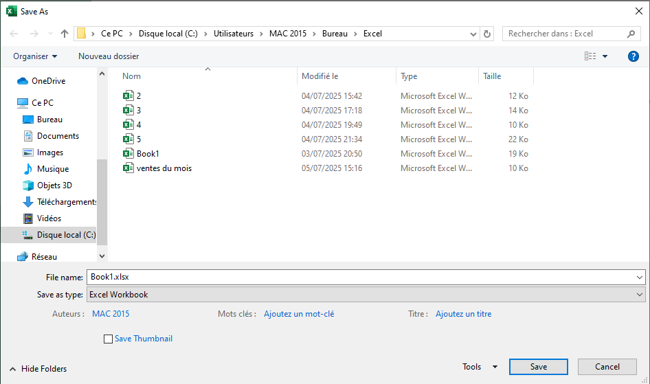
- In the File type list, click the format you want. Click the arrows to scroll through formats not immediately visible.
In the File name box, either accept the suggested name or type a new name for the workbook.
Excel File Formats
Format Extension Description Excel Workbook .xlsx Default XML-based format for Excel 2007–2019. Does not support VBA macros or Excel 4.0 macro sheets (.xlm). Strict Open XML Spreadsheet .xlsx ISO strict version of the Excel workbook (.xlsx) file format. Excel Macro-Enabled Workbook .xlsm XML-based file format that supports macros for Excel 2007–2019. Stores VBA macro code or Excel 4.0 macro sheets (.xlm). Excel Binary Workbook .xlsb Binary file format (BIFF12) for Excel 2007–2019. Excel Template .xltx Default template file format for Excel 2007–2019. Does not support VBA macros or Excel 4.0 macro sheets (.xlm). Macro-Enabled Template .xltm File format supporting macros for Excel templates in Excel 2007–2019. Stores VBA macro code or Excel 4.0 macro sheets (.xlm). Excel 97–2003 Workbook .xls Binary file format for Excel 97–2003 (BIFF8). Excel 97–2003 Template .xlt Binary template file format for Excel 97–2003 (BIFF8). Excel 5.0/95 Workbook .xls Binary file format for Excel 5.0/95 (BIFF5). XML Spreadsheet 2003 .xml XML Spreadsheet format (XMLSS). XML Data .xml XML data format. Excel Add-in .xlam XML-based add-in format that supports macros for Excel 2007–2019. An add-in is a supplemental program to run additional code. Supports VBA projects and Excel 4.0 macro sheets (.xlm). Excel 97–2003 Add-in .xla Add-in program to run additional code. Supports VBA projects. Excel 4.0 Workbook .xlw Excel 4.0 format that only stores worksheets, chart sheets, and macro sheets. You can open but not save to this format in Excel 2019. Text File Formats
Format Extension Description Formatted Text (space-delimited) .prn Space-delimited Lotus format. Saves only the active sheet. Text (tab-delimited) .txt Saves a workbook as a tab-delimited text file for use with another Microsoft Windows OS and ensures proper interpretation of tabs, page breaks, etc. Saves only the active sheet. Text (Macintosh) .txt Saves as a tab-delimited text file for use on Macintosh. Ensures proper interpretation of tabs, page breaks, etc. Saves only the active sheet. Text (MS-DOS) .txt Tab-delimited format for MS-DOS systems. Saves only the active sheet. Unicode Text .txt Saves workbook as Unicode text (character encoding standard by Unicode Consortium). CSV (comma-delimited) .csv Saves a workbook as comma-separated values for use with another Windows OS. Saves only the active sheet. CSV (Macintosh) .csv Saves as comma-separated values for Macintosh. Saves only the active sheet. CSV (MS-DOS) .csv Comma-delimited for MS-DOS systems. Saves only the active sheet. DIF .dif Data Interchange Format. Saves only the active sheet. SYLK .slk Symbolic Link format. Saves only the active sheet. Note: If you save a workbook in text format, all formatting will be lost.
Other File Formats
Format Extension Description DBF 3, DBF 4 .dbf dBase III and IV. You can open, but not save to this format in Excel. OpenDocument Spreadsheet .ods You can save Excel 2010 files in OpenDocument format (e.g. Google Docs, OpenOffice Calc). Formatting may be lost when saving/opening .ods files. PDF .pdf Portable Document Format. Retains document formatting and allows file sharing. Ideal for online viewing or professional printing. Cannot be easily edited. XPS Document .xps XML Paper Specification. Preserves formatting and is shareable. Ensures consistent appearance and protects content from easy modification. Clipboard File Formats
If you’ve copied data from the Clipboard in one of the following formats, you can paste it into Excel using Paste or Paste Special (Home / Clipboard / Paste).Format Extension Clipboard Type Identifiers Picture .wmf or .emf WMF or EMF image formats. Note: Excel converts WMF images pasted from other programs to EMF format. Bitmap .bmp Bitmap (BMP) image format. Excel File Formats .xls Binary formats for Excel 5.0/95 (BIFF5), Excel 97–2003 (BIFF8), Excel 2013 (BIFF12). SYLK .slk Symbolic Link format. DIF .dif Data Interchange Format. Text (tab-delimited) .txt Tab-delimited text format. CSV (comma-delimited) .csv Comma-separated values format. Formatted Text (*.prn) .rtf Rich Text Format (RTF). Excel only. Embedded Object .gif, .jpg, .doc, .xls, .bmp Microsoft Excel objects, OLE 2.0 compatible programs, images, or other presentation formats. Linked Object .gif, .jpg, .doc, .xls, .bmp OwnerLink, ObjectLink, Link, Picture, or other formats. Office Drawing Object .emf Office Drawing or Picture format (EMF). Text .txt Display Text, OEM Text. Single File Web Page .mht, .mhtml Web page with embedded media, applets, links, and referenced content. Web Page .htm, .html HTML format (Hypertext Markup Language). Note: When copying text from another program, Excel pastes it in HTML format regardless of the original format. Set a Print Area in Excel
A print area is a range of cells to include in the final printout. If you don’t want to print the entire worksheet, define a print area that includes only your selected data. When you press Ctrl + P or click the Print button on a worksheet with a defined print area, only that area will be printed. You can select multiple print areas on a single worksheet, and each area will print on a separate page. Saving the workbook also saves the print area.
Defining a print area gives you more control over how each printed page looks, and you should always set a print area before sending a worksheet to the printer. Without it, you may end up with cluttered, hard-to-read pages where important rows and columns are cut off, especially if your worksheet is larger than the paper size you’re using.
How to Set the Print Area
To tell Excel which section of your data should appear on a printed copy, use one of the following methods. The fastest way to define a fixed print range is:
- Select the part of the worksheet you want to print.
- On the Page Layout tab, in the Page Setup group, click Print Area > Set Print Area.
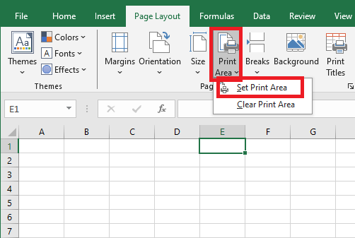
A faint gray line will appear to indicate the print area.
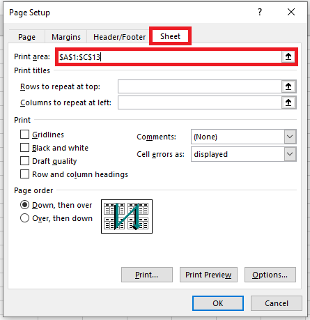
Want to see all your settings? Here’s a more transparent approach to setting a print area:
- Under the Page Layout tab, in the Page Setup group, click the dialog box launcher. This opens the Page Setup dialog box.
- Under the Sheet tab, place the cursor in the Print area field and select one or more ranges in your worksheet. To select multiple ranges, remember to hold down the Ctrl key.
- Click OK.
Tips and Notes:
- When you save the workbook, the print area is saved too. Every time you send the worksheet to the printer, only that area will be printed.
- To ensure the defined areas are exactly what you want, press Ctrl + P and preview each page.
- To quickly print a specific portion of your data without setting a print area, select the desired range(s), press Ctrl + P, and choose Print Selection from the dropdown just under Settings.
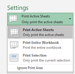
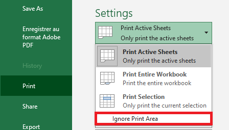
How to Force Excel to Ignore the Print Area
If you want a hard copy of the entire worksheet or workbook but don’t want to bother clearing all print areas, simply tell Excel to ignore them:
- Click File > Print or press Ctrl + P.
- Under Settings, click the arrow next to Print Active Sheets and select Ignore Print Area.
How to Print Multiple Areas on One Page
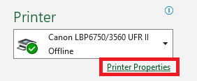
The ability to print multiple areas per sheet of paper is controlled by the printer driver, not by Excel. To check if this option is available:
- Press Ctrl + P, click on Printer Properties, and browse through the tabs in the Printer Properties dialog box looking for an option like Pages per Sheet.
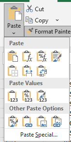
If your printer has such an option, you’re in luck. If not, the only workaround I can suggest is to copy the print ranges to a new sheet. Using the Paste Special function, you can link the copied ranges to the original data like this:
- Select the first print area and press Ctrl + C to copy it.
- On a new sheet, right-click any blank cell and choose Paste Special > Linked Picture (also called Paste as Linked Image).
- Repeat steps 1 and 2 for the other print areas.
- On the new sheet, press Ctrl + P to print all the copied print areas on a single page.
Displaying Formulas in Excel
If you are working on a worksheet containing numerous formulas, it can become difficult to understand how all these formulas are related to each other. Displaying formulas in Excel instead of results can help you track the data used in each calculation and quickly identify errors in your formulas. When you enter a formula into a cell and press the Enter key, Excel immediately displays the calculated result. To display all formulas in the cells that contain them, use one of the following methods.
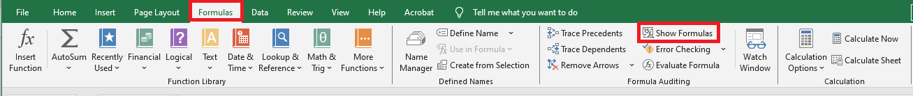
Display Formulas from the Excel Ribbon
In your Excel worksheet, go to the Formulas tab and, in the Formula Auditing group, click the Show Formulas button. Microsoft Excel will immediately display the formulas in the cells instead of their results. To revert to calculated values, click the Show Formulas button again to deactivate it.
Display Formulas from Excel Options Box
Go to File / Options. Select Advanced in the left pane, scroll down to the Display options for this worksheet section, and check the option Show formulas in cells instead of their calculated results.
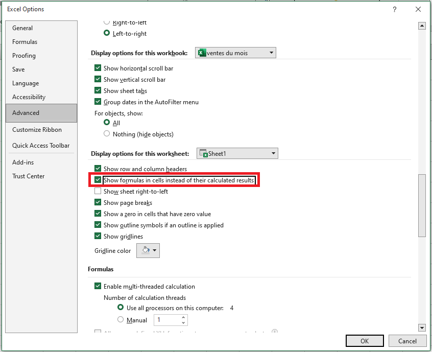
At first glance, this may seem like a longer path, but you may find it useful when you want to show formulas in several Excel sheets in the currently opened workbooks. In this case, you simply need to select the sheet name from the drop-down list and check the option Show formulas in cells… for each sheet.
NOTE:
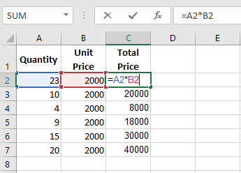
Regardless of the method you use above, Microsoft Excel will display all formulas in the current worksheet. To display formulas in other sheets and workbooks, you will need to repeat the process for each sheet individually.If you want to display the data used in a formula’s calculation, use one of the above methods to show formulas in the cells, then select the cell containing the formula in question, and you will see a result similar to the following:
If you click on a cell with a formula, but the formula does not appear in the formula bar, it is most likely that the formula is hidden and the worksheet is protected.
Adjusting Zoom Using Zoom Tools in Excel
Sometimes you zoom in on an Excel worksheet to better organize its layout. Other times, you zoom out to get an overview of certain values.
There are four methods available to adjust the zoom level in Excel.Method 1: Using IntelliMouse
By default, scrolling the mouse wheel moves the worksheet up or down. But you can use it to zoom in or out on the worksheet.
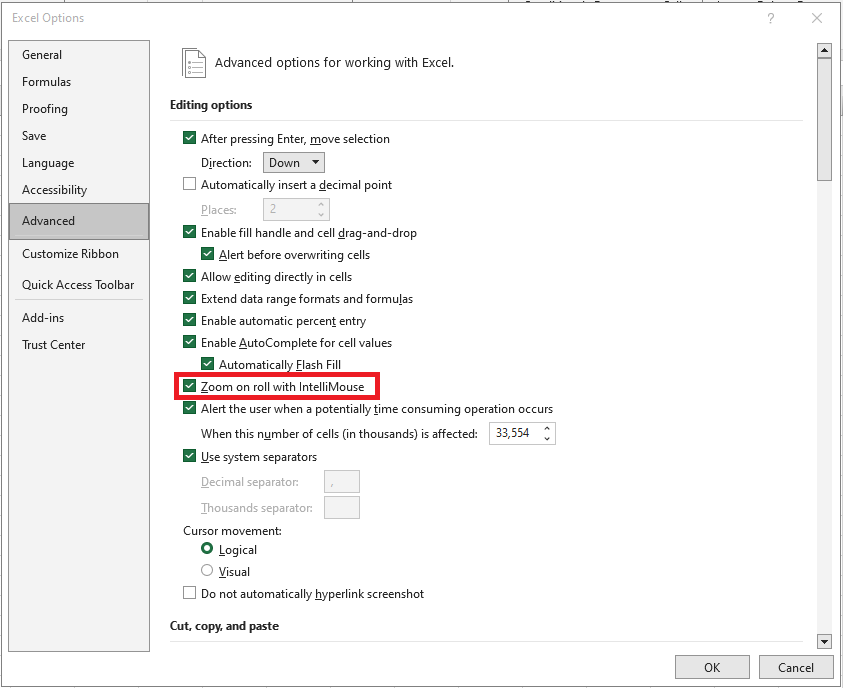
- Click the File tab on the ribbon
- Click Options
- In the Excel Options window, go to the Advanced tab
- Under Editing options, check Zoom on roll with IntelliMouse
- Click OK
Now, when you scroll the mouse wheel:
- Scrolling up zooms in
- Scrolling down zooms out
The zoom changes in 15% increments.
Note: With this feature enabled, the scroll wheel no longer moves the worksheet. If you want to move through the worksheet, refer to our previous article on 3 practical ways to navigate a worksheet in Excel.
To disable this feature later, just uncheck the same box in Step 4.
Method 2: Using the Zoom Slider
Instead of using IntelliMouse, you can also use the zoom slider found in the bottom-right corner of the Excel window.
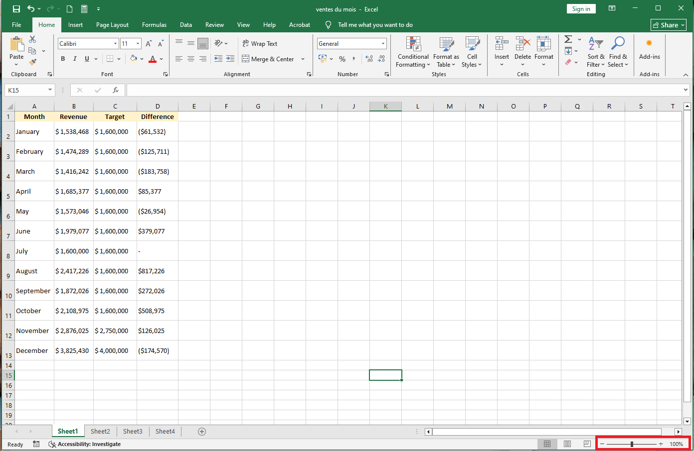
Click the Zoom Out or Zoom In buttons to change the view (each click adjusts the zoom by 10%)- You can also click anywhere on the slider itself
- The center point (middle of the slider) represents 100% zoom
- Clicking to the right zooms in
- Clicking to the left zooms out
You can also click on Zoom Level to manually adjust the zoom.
When you click Zoom Level, a dialog box appears where you can:
- Choose a preset zoom level
- Enter a custom percentage
- Choose Fit Selection, which zooms in to make the selected range fill the screen
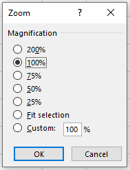
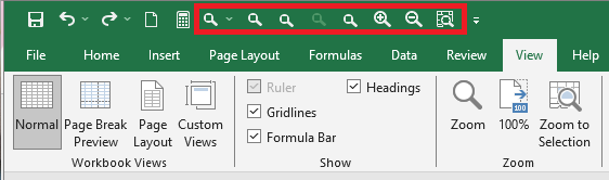
Method 3: Using the View Tab Toolbar
You can also change the zoom level using the View tab on the ribbon.
Under the Zoom group, there are three options:
- Zoom: Opens the same dialog box as the Zoom Level button
- 100%: Immediately sets the zoom level to 100%
- Zoom to Selection: Zooms in to make the selected range fill the screen (same as « Fit Selection » in the Zoom dialog)
So, the toolbar offers a quick way to manage zoom.
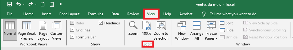
Method 4: Adding Zoom Buttons to the Quick Access Toolbar
If you prefer to customize the Quick Access Toolbar, you can also add zoom-related buttons there:
- Click the downward arrow at the end of the Quick Access Toolbar
- Select More Commands… from the dropdown
- In the Choose commands from dropdown, select All Commands
- Scroll through the list to find the zoom-related buttons
- The 100% button is located near the beginning
- Six other zoom buttons are found near the end of the list
- For each button, click Add to place it on the Quick Access Toolbar
- After adding the necessary buttons, click OK to confirm
You now have dedicated zoom buttons available at all times in the Quick Access Toolbar.
Editing Document Properties in Excel
Types of Document Properties
Before learning how to view, edit, and delete document properties (metadata) in Excel, let’s clarify the types of properties an Office document can have:
- Type 1: Standard Properties – These are common to all Office applications. They include basic information about the document such as Title, Subject, Author, Category, etc. You can assign your own text values to make documents easier to search on your PC.
- Type 2: Automatically Updated Properties – These include system-controlled data such as file size, creation/modification date, or application-specific properties such as page count, word count, or application version.
- Type 3: Custom Properties – These are user-defined properties that allow you to add additional metadata to your Office document.
- Type 4: Organization Properties – Specific to your organization.
- Type 5: Document Library Properties – These refer to documents stored in a document library on a website or public folder. The person who creates the library can define certain property fields and validation rules that must be filled or corrected before uploading files.
Viewing Document Properties
To find your document’s properties in Excel:
- Go to File > Info
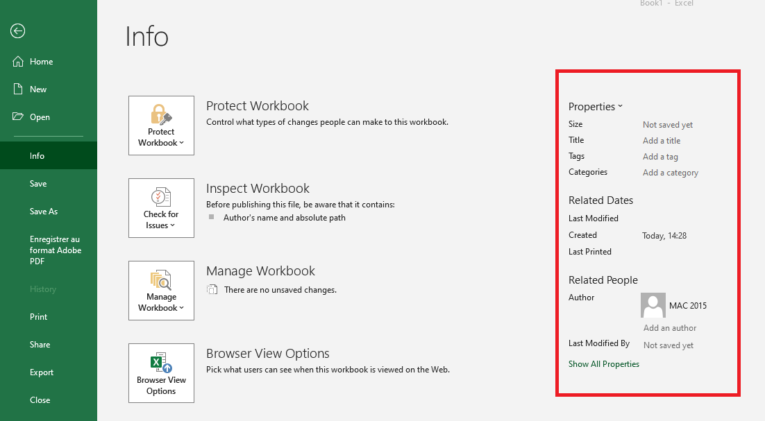
- Click on Properties > Advanced Properties
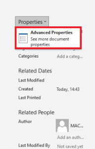
- The Properties dialog box will appear.
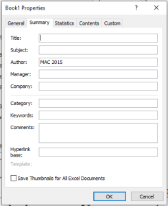
Here you can view general information, statistics, and content details. You can also edit the document summary or set custom properties.
Editing Document Properties
When viewing document properties, you can instantly add or correct information.
To add an author quickly:- Go to File > Info
- In the Related People section, hover over Add an author and click it
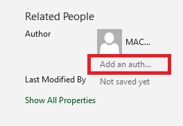
- Type the author’s name
- Click anywhere in the Excel window to save
You can also use this method to modify the title, tags, or category.
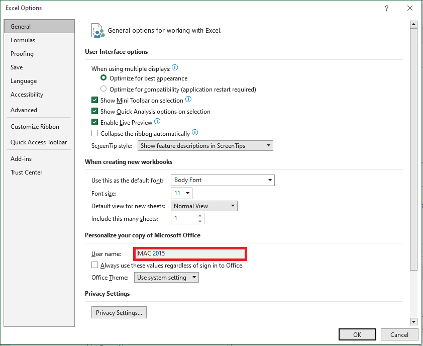
By default, Excel uses your Windows username as the document author. To change this:
- Click File > Options
- Select General on the left
- Scroll to Personalize your copy of Microsoft Office
- Enter your actual name in the User name field
- Click OK
Defining Custom Properties
To add custom document properties:
- Go to File > Info
- Click Properties > Advanced Properties
- In the dialog box, go to the Custom tab
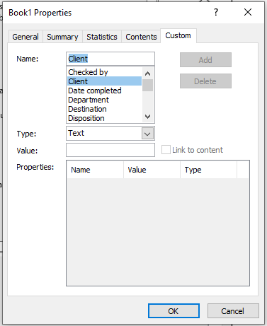
- Enter a name or select one from the predefined list
- Choose the data type
- Enter a value
- Click Add
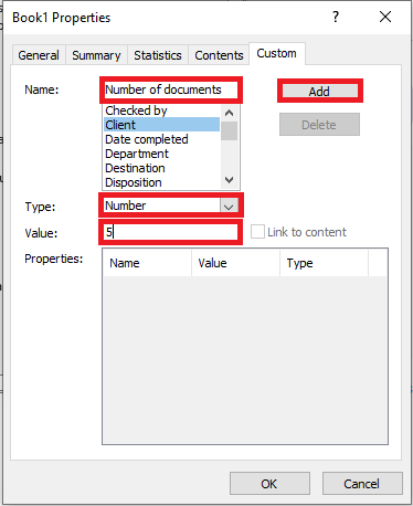
NOTE:
The value format must match your selection in the Type list. This means that if the selected data type is Number, you must enter a number in the Value field. Values that do not match the property type are saved as text.- The custom property will appear in the list. Click OK to save.
The value must match the selected data type (e.g., numbers for number fields). If not, the value will be saved as text.
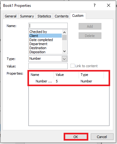
To remove a custom property, select it in the list and click Delete > OK.
To modify metadata beyond author, title, tags, and category:
- In the document panel, place your cursor in the desired field and edit.
- In the Properties dialog, switch to the Summary tab and update fields. Click OK—changes are saved automatically.
Deleting Document Properties
To remove your name or organization from document properties:
Use the Document Inspector
This tool scans your document for hidden data and personal info.
- Go to File > Info
- Click Check for Issues > Inspect Document
- The Document Inspector window opens. All checkboxes are selected by default—leave them checked.
- Click Inspect
- Once results appear, click Remove All under each category of interest—especially Document Properties and Personal Information
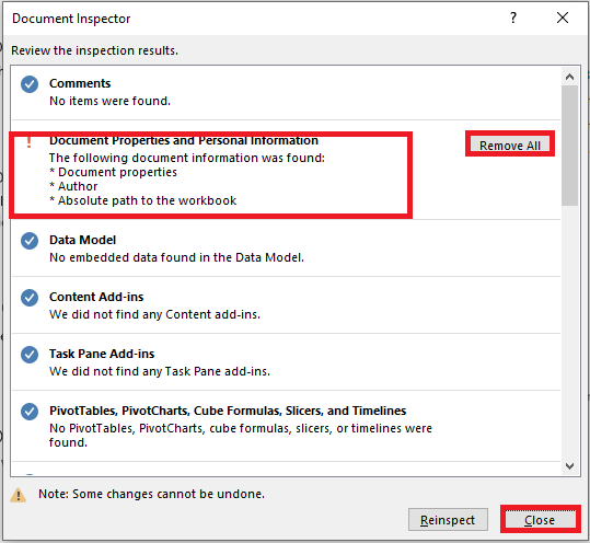
- Close the Inspector.
- (Recommended) Save the file under a new name to keep an original copy with metadata intact.
Remove Metadata from Multiple Files
To delete properties from several files at once using Windows Explorer:
- Open the folder containing the Excel files
- Select the desired files
- Right-click and choose Properties
- Go to the Details tab
- Click Remove Properties and Personal Information
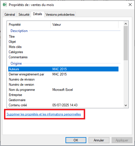
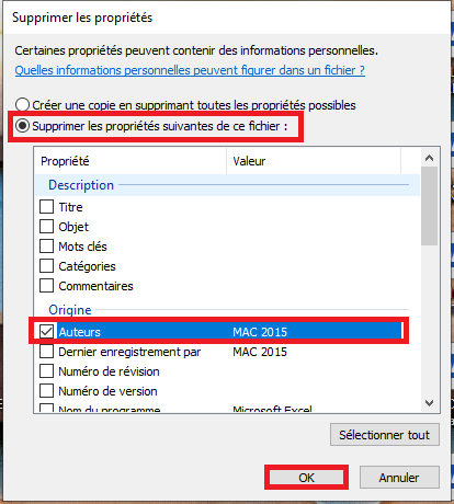
- Select Remove the following properties from this file
- Check specific fields or click Select All
- Click OK
Protect Document Properties
If you want to prevent others from modifying metadata:
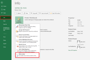
- Go to File > Info
- Click Protect Workbook (under the Permissions section)
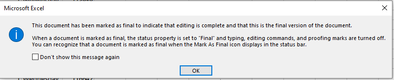
- Choose Mark as Final
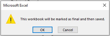
- A prompt will inform you that the document will be marked as final and uneditable. Confirm or cancel.
If you want to allow specific people to modify the workbook, you can set a password:
- Stay in Backstage view (File tab).
- Choose Save As
- At the bottom of the dialog, click Tools > General Options
- Enter a password in the Password to modify field
- Click OK
Figure 1.4.6-s: Protect Document Properties - Confirm the password
- Click OK
Figure 1.4.6-t: Protect Document Properties - Select a folder and click Save.
Your file is now protected from unwanted changes.
Note: Anyone with the password can remove it from the same dialog box, so it’s not completely tamper-proof.