Votre panier est actuellement vide !
Étiquette : pratical_excel
Changing Window Views in Excel
It is often very practical, or even necessary, to display multiple worksheets from the same workbook on screen at the same time:
- For example, when creating complex formulas that pull data from different sheets, you often need to switch back and forth between worksheets.
- Or when comparing data tables located in different sheets.
To compare several sheets simultaneously, without having to constantly switch between tabs, simply enable Excel’s multi-window mode by clicking the New Window button in the View tab on the ribbon:
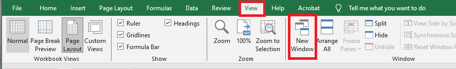
This creates a new instance of the currently open workbook.
Each window instance is easily identifiable by the number that appears after the filename in the title bar (at the top of the Excel window).
You can then rearrange the windows so they are visible on the screen at the same time:
- Either manually using your mouse (if your windows are not maximized),
- Or by clicking the View Side by Side button.
Side by Side View
It’s possible to scroll both windows simultaneously.
To do this, simply click the Synchronous Scrolling button.
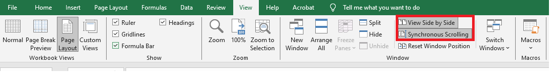
NOTE:
The Synchronous Scrolling feature is only available when Side by Side view is enabled.
If you adjust the size of a window and want to instantly go back to the previous layout from when you clicked View Side by Side, click the Reset Window Position button:
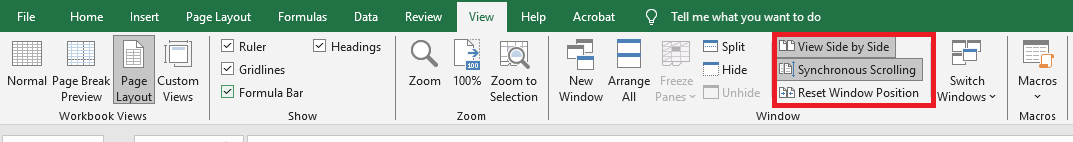
The Side by Side view is very convenient for comparing the content of two worksheets.
However, it is limited to displaying only two windows at the same time.
Automatic Window Arrangement
To display more than two windows at once, you’ll need to use another Excel feature:
Arrange All
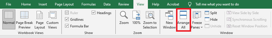
This feature automatically arranges all open windows.
(To limit the arrangement to windows of the current workbook only, check Windows of active workbook.)
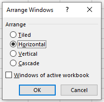
Here are the available layout options:
- Tiled: Uses all available screen space to display windows in a tiled layout (divided horizontally and vertically).
- Horizontal: Displays windows in horizontal rows.
Due to the large space taken up by the ribbon, this is the least practical layout.
As shown below, the interface may occupy the entire screen, leaving no room for worksheet content. - Vertical: Displays windows in vertical columns.
- Cascade: Displays windows almost maximized, one over the other in a cascading layout.
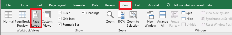
Change Workbook Views in Excel
Excel offers three workbook views: Normal, Page Layout, and Page Break Preview.
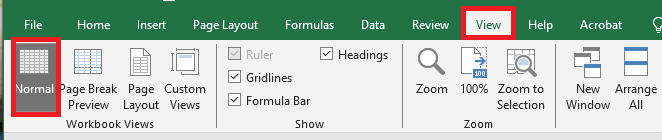
Normal View
You can return to Normal View at any time.
- On the View tab, in the Workbook Views group, click Normal.
Result:
If you switch to another view and then return to Normal View, Excel may display page breaks. To hide these page breaks, close and reopen the Excel file.
To permanently hide page breaks for that worksheet:
- Go to File > Options > Advanced
- Scroll down to Display options for this worksheet
- Uncheck Show page breaks
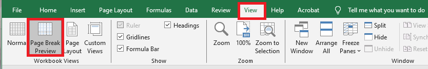
Page Break Preview
Page Break Preview gives you a good overview of where pages will break when printing your document.
Use this view to easily click and drag page breaks.- On the View tab, in the Workbook Views group, click Page Break Preview.
Result:
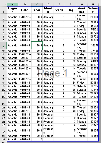
You can drag the page breaks to fit all your content onto a single page.
⚠️ Caution: Excel does not warn you if the print becomes unreadable.By default, Excel prints down first, then over.
In other words, it prints all rows in the first set of columns, then all rows in the next set of columns, and so on.Page Layout View
Use Page Layout View to see where pages begin and end, and to add headers and footers.
- On the View tab, in the Workbook Views group, click Page Layout.
Result:

Customize the Quick Access Toolbar in Excel
Accessing the commands you use most often should be easy. That’s exactly what the Quick Access Toolbar is designed for. Add your favorite commands to the Quick Access Toolbar so they are just one click away, regardless of which ribbon tab is currently open.
What is the Quick Access Toolbar?
The Quick Access Toolbar is a small customizable toolbar located at the top of the Office application window that contains a set of frequently used commands. These commands are accessible from nearly any part of the application, regardless of which ribbon tab is currently selected.
The Quick Access Toolbar has a dropdown menu that includes a predefined set of default commands, which can be shown or hidden. Additionally, it provides an option to add your own commands.
There’s no hard limit to how many commands you can add to the Quick Access Toolbar, though not all may be visible depending on your screen size.
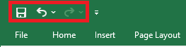
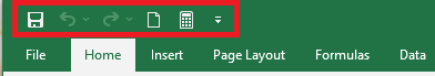
Where is the Quick Access Toolbar in Excel?
By default, the Quick Access Toolbar is located in the top-left corner of the Excel window, above the ribbon. If you prefer having it closer to the worksheet area, you can move it below the ribbon.
Customizing the Quick Access Toolbar
By default, the Excel Quick Access Toolbar contains only three buttons: Save, Undo, and Redo. If you frequently use other commands, you can also add them to this toolbar.
These instructions apply to Excel, but they work the same for other Office applications like Outlook, Word, PowerPoint, etc.
You can customize the Quick Access Toolbar by:
- Adding your own commands
- Changing the order of both default and custom commands
- Displaying the toolbar in one of two available locations
- Adding macros
- Exporting and importing your customization settings
Limitations:
- You can only add commands to the toolbar. Individual list items (like spacing values) and individual styles can’t be added—only the entire list or gallery.
- Only command icons can be shown, not text labels.
- You can’t resize toolbar buttons. The only way to change their size is by changing your screen resolution.
- The toolbar cannot be displayed on multiple lines. If you add more commands than there is space for, some will be hidden. To access them, click the More Commands button.
Accessing the Customize Quick Access Toolbar Window
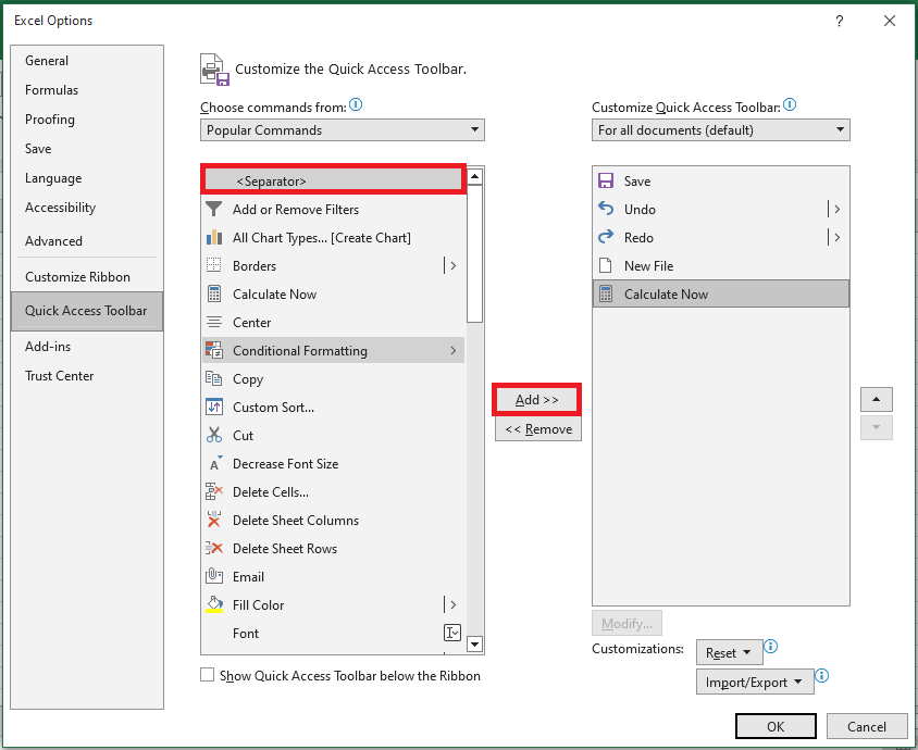
Most customizations are made from the Customize the Quick Access Toolbar window, found in the Excel Options dialog.
You can access it in several ways:
- Go to File > Options > Quick Access Toolbar
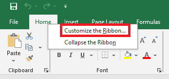
- Right-click anywhere on the ribbon and choose Customize the Quick Access Toolbar…
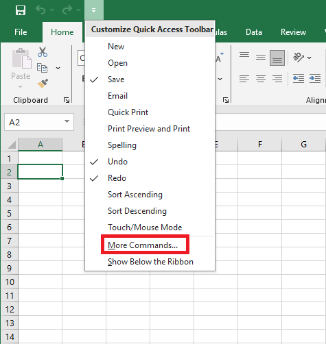
- Click the Customize Quick Access Toolbar button (the downward arrow at the far right), then select More Commands…

This opens the dialog where you can add, remove, and rearrange toolbar commands.
Adding a Command Button to the Quick Access Toolbar
Depending on the type of command, you can add it in one of three ways:
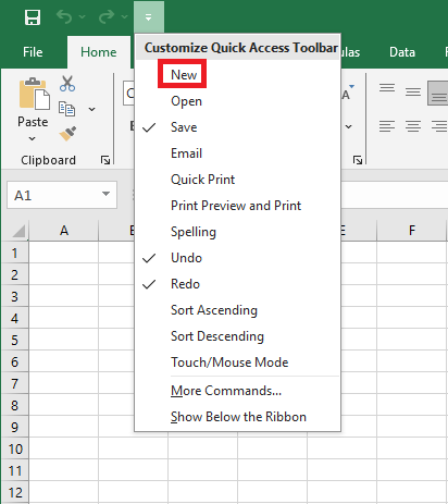
Enable a Command from the Predefined List
- Click the Customize Quick Access Toolbar button (downward arrow).
- From the list of commands, click the one you want to enable.
For example, to create a new worksheet with one click, select New, and the button will appear in the toolbar.
Add a Ribbon Button to the Quick Access Toolbar
- Right-click the desired ribbon command.
- Select Add to Quick Access Toolbar from the context menu.
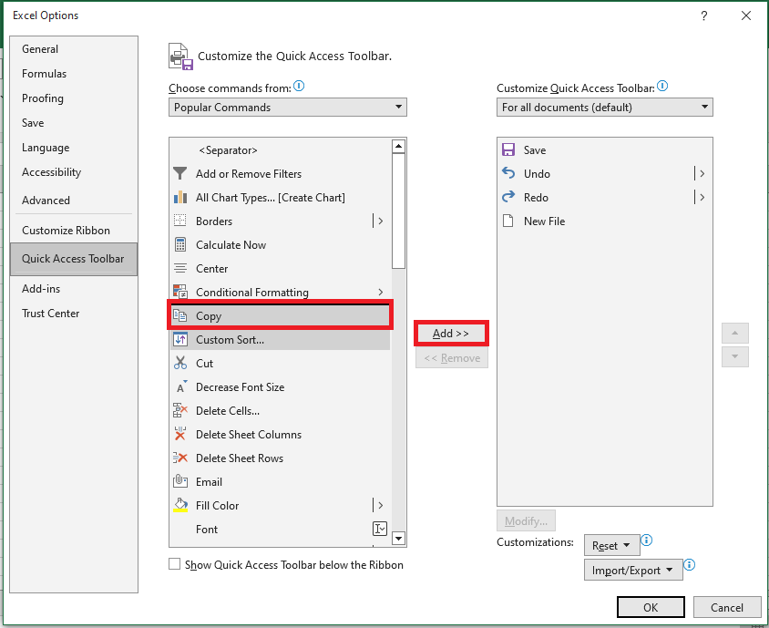
Add a Command Not on the Ribbon
- Right-click the ribbon and choose Customize the Quick Access Toolbar…
- In the Choose commands from dropdown, select Commands Not in the Ribbon
- From the list on the left, select the command to add
- Click Add
- Click OK to save
For example, to close all Excel windows with one click, you can add the Close All button.
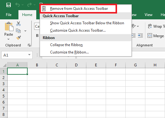
Removing a Command from the Quick Access Toolbar
To remove a command (default or custom), right-click it and select Remove from Quick Access Toolbar.
Or, open the Customize Quick Access Toolbar window, select the command, and click Remove.
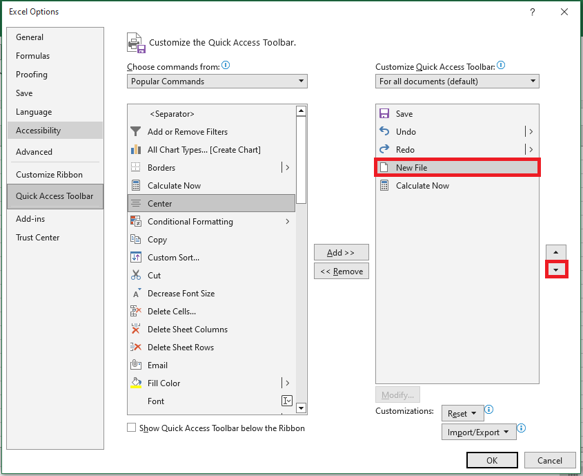
Rearranging Commands on the Quick Access Toolbar
To change the order of commands:
- Open the Customize Quick Access Toolbar window.
- On the right-hand list, select the command you want to move.
- Use the Up or Down arrow to change its position.
For example, to move the New File button to the far right, select it and click Move Down.
Grouping Commands on the Quick Access Toolbar
If your toolbar contains many commands, you may want to group them logically—e.g., separating default from custom commands.
Although you can’t create full command groups like on the ribbon, you can add separators:
- Open the Customize Quick Access Toolbar dialog.
- In the Choose commands from dropdown, select Popular Commands.
- In the command list, select and click Add.
- Use Move Up or Move Down to place it where you want.
- Click OK to save.
Therefore, the Quick Access Toolbar appears to have two sections.
Moving the Quick Access Toolbar Above or Below the Ribbon
By default, the Quick Access Toolbar is placed above the ribbon. If you prefer to have it below, follow these steps:
- Click the Customize Quick Access Toolbar button.
- In the dropdown menu, select Show Below the Ribbon.
To move it back to the top, click the same button again and select Show Above the Ribbon.
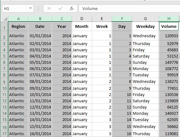
Hiding or Displaying Columns and Rows in Excel
Sometimes, it can be useful to hide columns or rows in Excel.
Hiding Columns and Rows
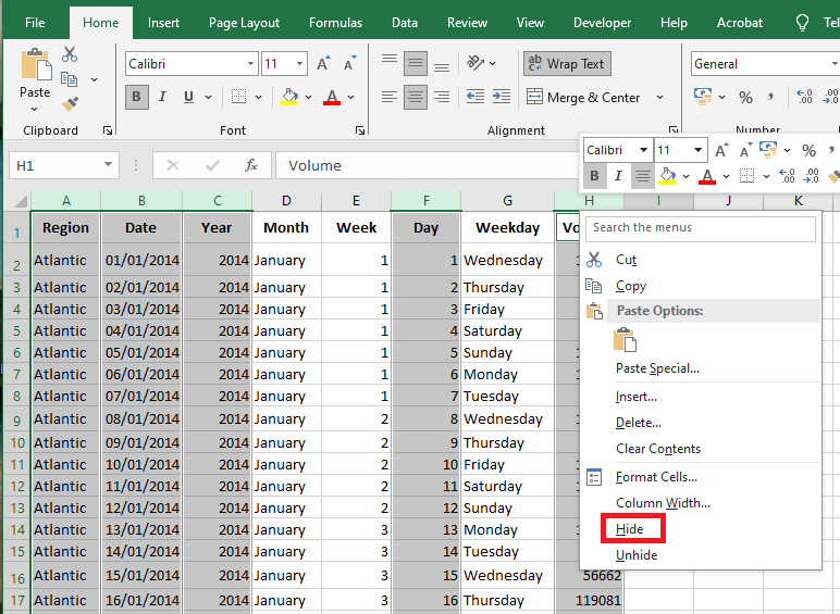
To hide a column, follow these steps:
- Select a column.

- Right-click, then click Hide.
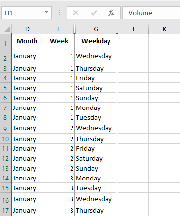
Result:
To hide a row, select the row, right-click, then click Hide.
Displaying Columns and Rows
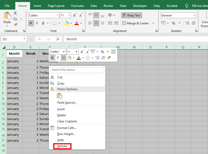
To unhide a column, follow these steps:
- Select the columns on either side of the hidden column.
- Right-click, then click Unhide.
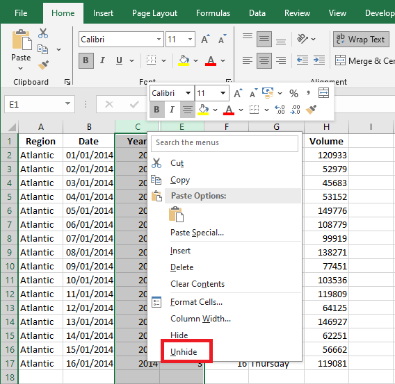
Result:
To unhide a row, select the rows on either side of the hidden row, right-click, then click Unhide.
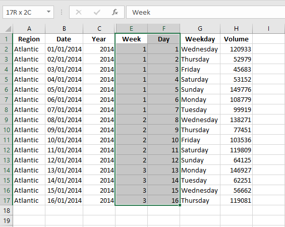
Multiple Columns or Rows
To hide multiple columns, follow these steps:
- Select multiple columns by clicking and dragging over the column headers.
- To select non-adjacent columns, hold down Ctrl while clicking on the column headers.
- Right-click, then click Hide.
Result:
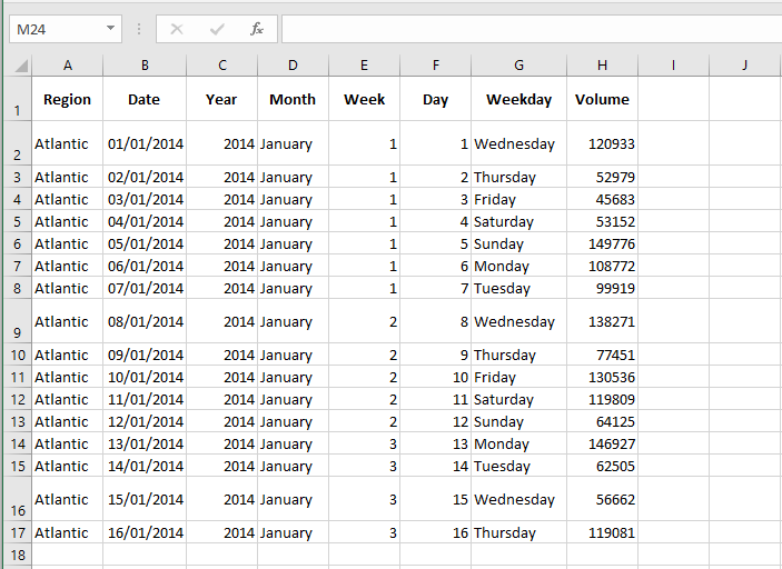
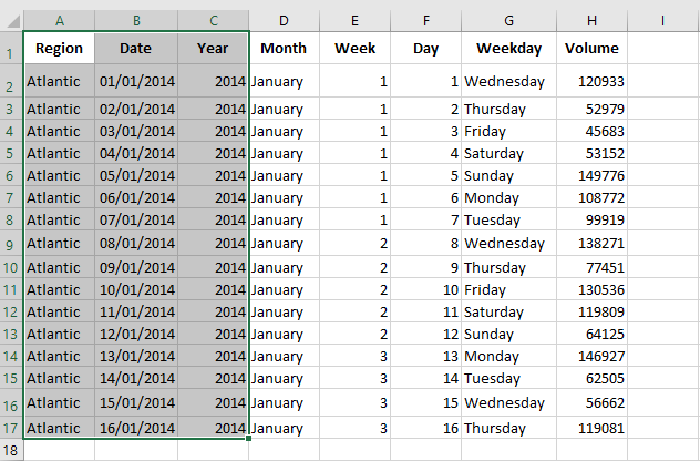
- To unhide all columns, follow these steps:
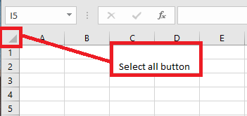
Select all columns by clicking the Select All button.
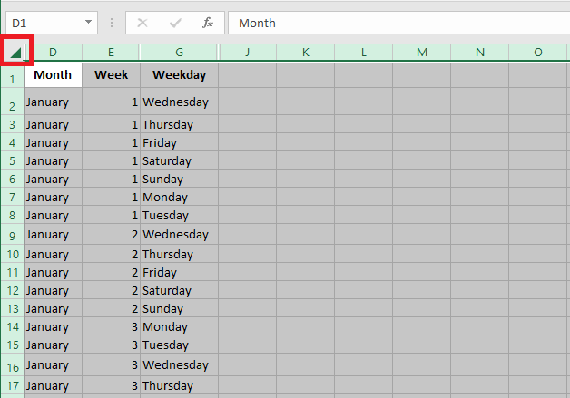
Right-click on any column header, then click Unhide.
Result: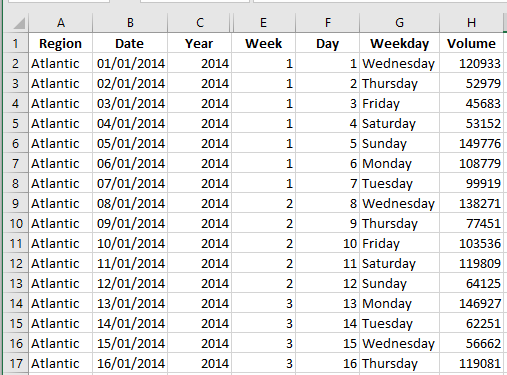
Tips and Tricks for Hiding and Displaying Rows
As you’ve just seen, hiding and unhiding rows in Excel is simple and quick. However, in some situations, even a simple task can become tricky. Below are simple solutions to a few common issues.
Hiding Rows Containing Blank Cells
To hide rows containing blank cells, proceed as follows:
- Select the range that contains the blank cells you want to hide.
- On the Home tab, in the Editing group, click Find & Select > Go To Special.
- In the Go To Special dialog box, select Blanks and click OK. This will select all the blank cells in the range.
- On the Home tab, in the Cells group, select Format > Hide & Unhide > Hide Rows to hide the rows that contain blank cells.
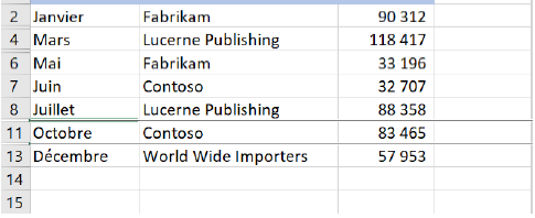
This method works well when you want to hide all rows containing at least one blank cell, as shown in the screenshot below:
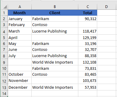
Result:
Locating All Hidden Rows in a Sheet
If your worksheet contains hundreds or thousands of rows, it can be difficult to detect which ones are hidden. The following trick makes it easy:
- On the Home tab, in the Editing group, click Find & Select > Go To Special.
- In the Go To Special window, select Visible cells only and click OK.
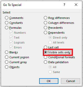
This will select all visible cells and mark the rows adjacent to hidden rows with a white border.
Copying Visible Rows in ExcelSuppose you’ve hidden a few irrelevant rows and now want to copy only the relevant visible data into another sheet or workbook. How would you proceed?
If you select the visible rows with the mouse and press Ctrl + C, the hidden rows will also be copied!To copy only visible rows in Excel, do the following:
- Select the visible rows using the mouse.
- Go to the Home tab, in the Editing group, and click Find & Select > Go To Special.
- In the Go To Special window, select Visible cells only, then click OK. This will select only the visible rows as described in the previous tip.
- Press Ctrl + C to copy the selected rows.
- Press Ctrl + V to paste the visible rows.
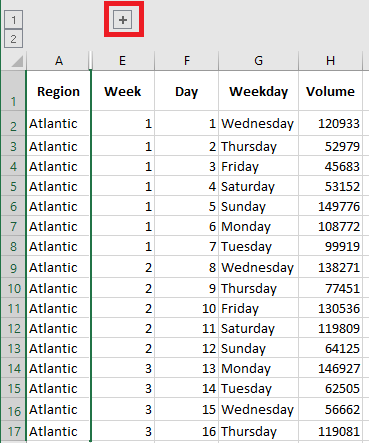
Hiding and Displaying Columns Using a Button
To hide and unhide columns by clicking a button, follow these steps:
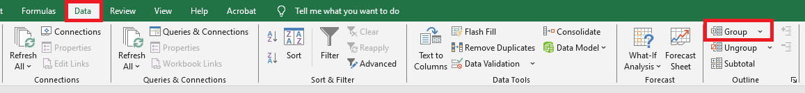
- Select one or more columns.
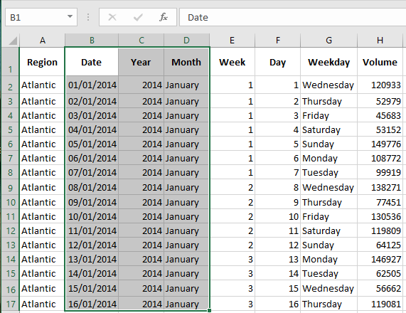
- On the Data tab, in the Outline group, click Group.
- To hide the columns, click the minus sign.
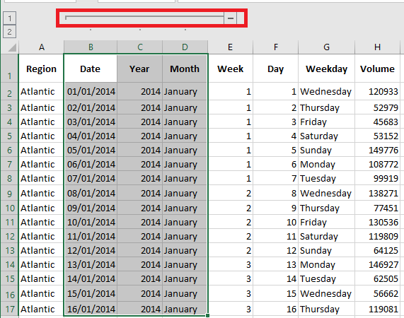
- To unhide the columns again, click the plus sign.
To ungroup the columns, first select them, then on the Data tab, in the Outline group, click Ungroup.
Hiding Cells
Finally, to hide cells in Excel, follow these steps:
- Select a range of cells.
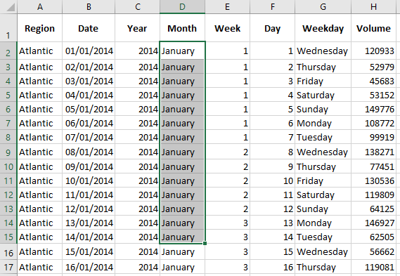
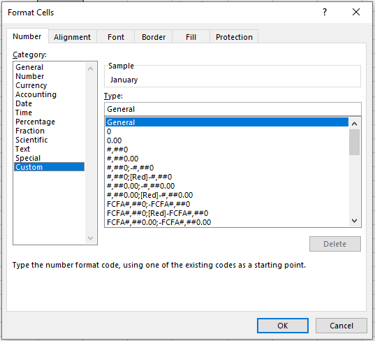
- Right-click, then click Format Cells. The Format Cells dialog box appears.
- Select Custom.
- Enter the following number format code:
;;; - Click OK.
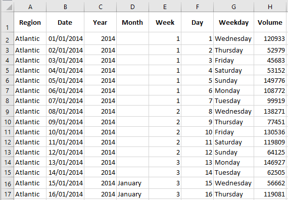
Result:
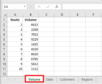
Hiding or Displaying Worksheets in Excel
Hiding worksheets can be a simple way to protect data in Excel or just a way to reduce clutter from certain tabs. Below are a few very simple methods to hide and unhide worksheets and workbooks in Excel.
Hiding a Worksheet
Select the worksheet you want to hide by clicking on its tab at the bottom. By holding the Ctrl key while clicking, you can select multiple tabs at once.
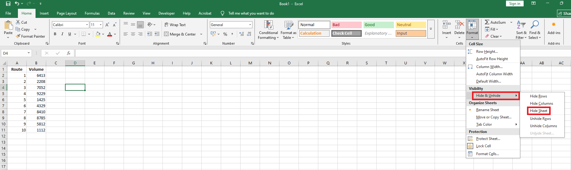
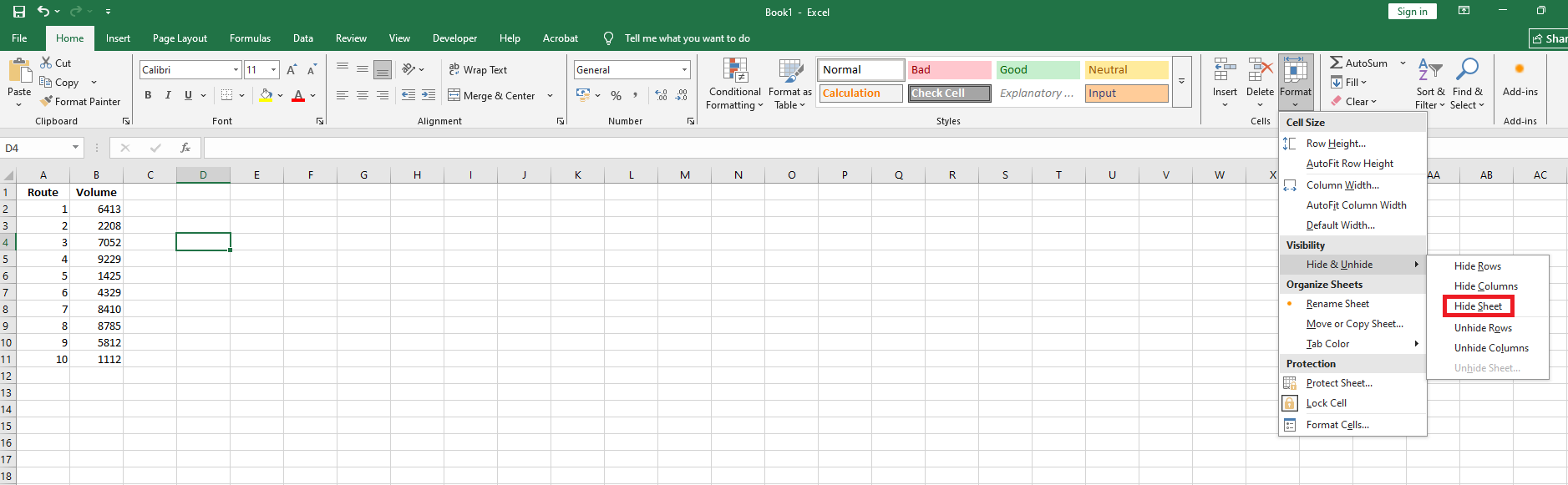
On the Home tab, click Format, located in the Cells group. Under Visibility, select Hide & Unhide, then choose Hide Sheet.
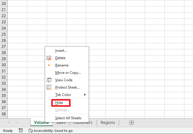
You can also simply right-click on the tab and select Hide.
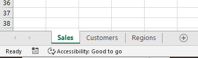
Your worksheet will no longer be visible; however, the data contained in the hidden worksheet can still be referenced from other worksheets.
Unhiding a Worksheet
To unhide a worksheet, simply do the reverse.
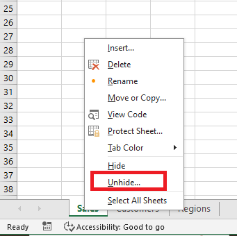
On the Home tab, click Format in the Cells group, then under Visibility, select Hide & Unhide, and choose Unhide Sheet.
Or, you can right-click on any visible tab and select Unhide.
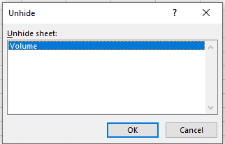
In the Unhide pop-up window, select the worksheet you want to display and click OK.NOTE:
Although you can hide multiple sheets at once, you can only unhide one sheet at a time.
Hiding a Worksheet with Visual Basic
While the regular Hide mode is convenient, it is not highly secure. If you want to increase the level of protection, there is also a Very Hidden mode.
To access the Very Hidden setting, you need to use the built-in Visual Basic Editor by pressing Alt + F11.Select the worksheet you want to hide from the dropdown list under Properties, or by clicking once on the worksheet in the VBAProject window. Then, set the Visible property to 2 – xlSheetVeryHidden.
Close the Visual Basic Editor when you are done.
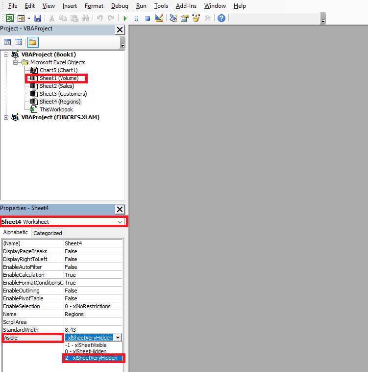
When the Very Hidden attribute is set on a worksheet, the Unhide Sheet option remains unavailable in the Format menu of the Home tab.
To remove the Very Hidden attribute and show the worksheet again, return to the Visual Basic Editor by pressing Alt + F11 once more and set the Visible property to 1 – xlSheetVisible.
Close the editor when done.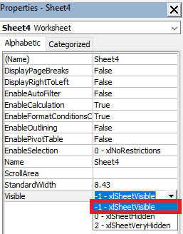
Inserting Headers and Footers in Excel
From the Insert Tab
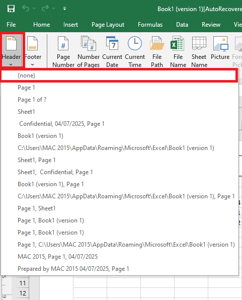
You can use a header to include the same information at the top of each printed page, or a footer to include information at the bottom of each page. You can enter your own custom headers or footers, insert built-in ones, or add specific elements such as images or page numbers.
To add a header or footer:
-
Click the Insert tab.
-
Click the Text button.
-
Select Header & Footer.
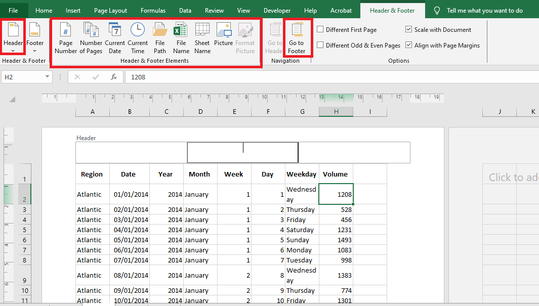
 The Header & Footer view appears, and the header section becomes active. Click in the header section where you want to add text.
-
Enter a custom text or select a predefined header from the Header & Footer Elements group or the Header dropdown menu.
-
To view the footer section, click the Go to Footer button.
-
Click in the footer section where you want to add text.
-
Enter custom text or select a predefined footer from the Header & Footer Elements group or the Footer dropdown menu.
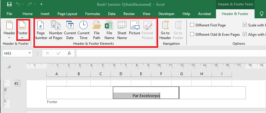
Headers and footers can be formatted using the commands in the Font group on the Home tab. The Header & Footer Elements group provides a variety of built-in options that you can use:
Button Description Page Number Displays the correct page number for each page Number of Pages Displays the total number of pages in the worksheet Current Date Displays the current date Current Time Displays the current time of day File Path Displays the file name and path of the workbook File Name Displays the name of the workbook Sheet Name Displays the name of the worksheet Picture Opens the Insert Picture dialog to insert an image file Format Picture Available after inserting a picture; lets you resize or adjust brightness/contrast From the Page Layout TabTo add a header and footer from the Page Layout tab:
-
Click the Page Layout tab.
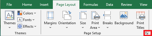
-
In the Page Setup section, click the Dialog Box Launcher on the bottom-right corner.
-
Click the Header/Footer tab.
-
Use the Header dropdown to choose a built-in header.
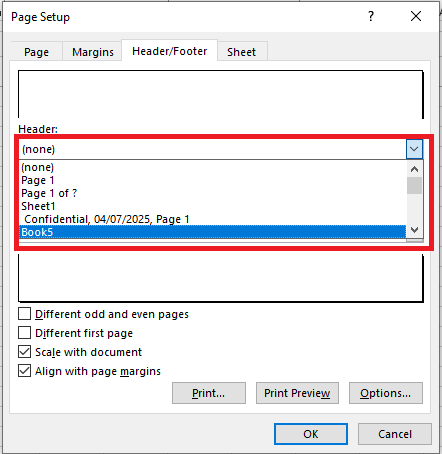
-
Use the Footer dropdown to choose a built-in footer.
-
Click the Custom Header button.
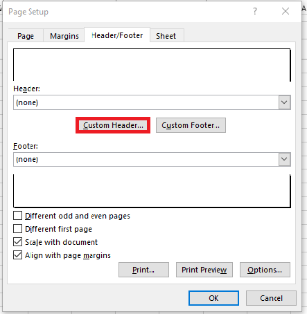
-
Click the Custom Footer button.
-
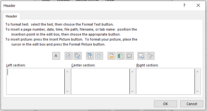
Select one of the sections (left, center, or right) to place the header or footer text.
-
Type your desired header or footer text.
-
Select the text and click the Format Text (A) button to apply font styling.
-
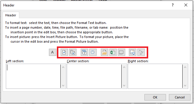
Click any of the buttons to insert a built-in element, including:
-
Insert Page Number
-
Insert Total Pages
-
Insert Date
-
Insert Time
-
Insert File Path
-
Insert File Name
-
Insert Sheet Name
-
Insert Picture
-
Click OK.
-
Click OK again.
Once completed, the header and footer will be applied to the worksheet you’re editing. If you do not see the changes, click the View tab, and under “Workbook Views,” click Page Layout.
How to Remove Headers and Footers
If you are tasked with editing and removing headers and footers from a document, you can do so in at least two ways.
From the Insert Tab
To remove the header and footer using the Insert tab:-
Open Microsoft Excel.
-
Open the document you want to modify.
-
Click the Insert tab.
-
In the Text section, click Header & Footer.
-
In the Header & Footer tools, click the Header button and select None.
-
Still under Text, click Header & Footer again if necessary.
-
In the Footer button, select None.
-
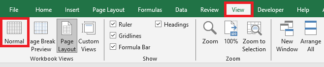
Click the View tab.
-
Under “Workbook Views,” click Normal to exit Page Layout view.
After completing these steps, the header and footer will be removed from your Excel worksheet.
From the Page Layout Tab
To remove the header and footer using the Page Layout tab:-
Open Microsoft Excel.
-
Open the document you want to customize.
-
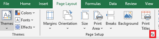
Click the Page Layout tab.
-
In the Page Setup section, click the Dialog Box Launcher on the right.
-
Click the Header/Footer tab.
-
From the Header dropdown, select None.
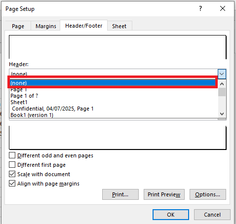
-
From the Footer dropdown, select None.
-
Click OK.
-
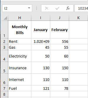
Adjusting Row Height and Column Width in Excel
If you find it necessary to increase or decrease the widths of columns or the heights of rows in Excel, there are several methods available to make these adjustments. The table below shows the minimum, maximum, and default sizes for each, based on a point scale.
Type Min. Max. Default Column 0 (hidden) 255 8.43 Row 0 (hidden) 409 15.00 NOTE:Pressing Ctrl+N also creates a new workbook using the Book.xltx template.
By default, Excel columns are 8.43 characters wide, but each individual column can be widened up to 255 characters. If the data entered in a cell is either wider or narrower than the default column width, you can adjust the column width to make it wide enough to display the data.
You can adjust column width manually or by using AutoFit.
To manually adjust column width:-
Position your mouse pointer on the right edge of the gray column header.
-
The pointer changes into a resizing tool (a double-headed arrow).
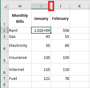
-
Drag the resizing tool to the left or right until the desired width is reached, then release the mouse button.
To automatically adjust column width:
-
Position your mouse pointer on the right edge of the column header.
-
The pointer changes into a resizing tool.
-
Double-click the border of the column header.
-
Excel automatically resizes the column, making it slightly wider than the widest cell entry it contains.
Adjusting row height works similarly to adjusting column width.
There will be times when you want to increase the height of a row to visually provide space above or below it.To adjust the height of a single row:
-
Position your mouse pointer on the bottom edge of the row header you want to adjust.
-
The pointer changes into a resizing tool.

-
Drag the resizing tool up or down until the desired height is reached, then release the mouse button.

To automatically adjust row height:
-
Position your mouse pointer on the bottom edge of the row header you want to adjust.
-
The pointer changes into a resizing tool.
-
Double-click to adjust the row height automatically based on the font size.
-
Excel automatically resizes the row, making it slightly taller than the tallest content within the row.
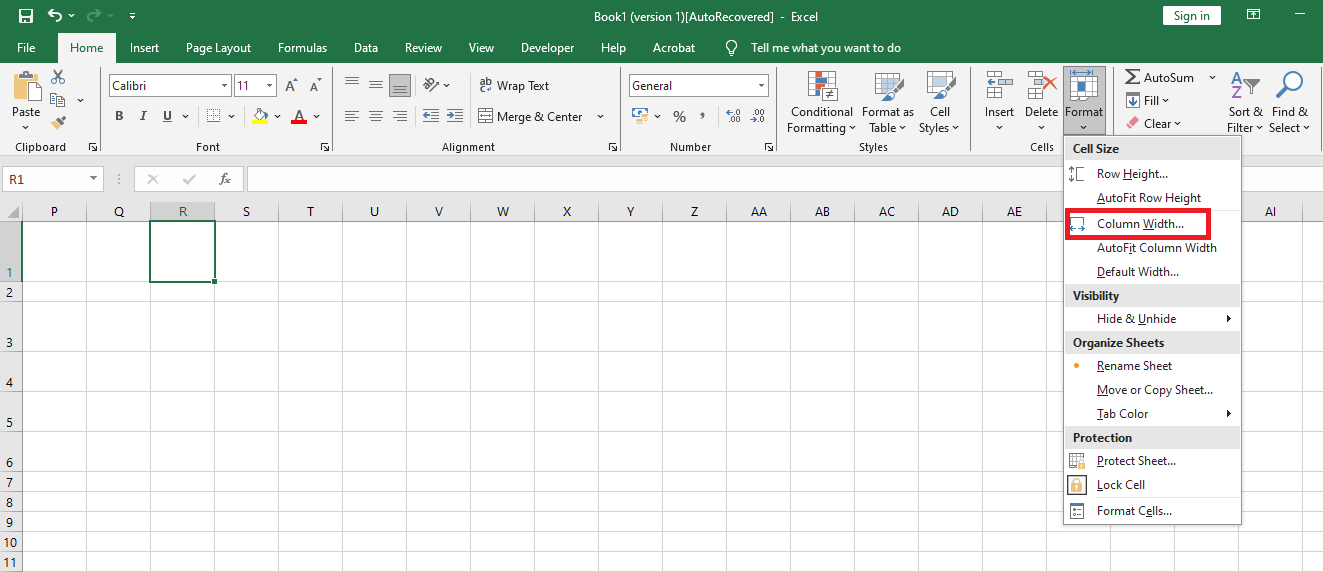
To set a specific column width:
-
Select the column(s) you want to modify.
-
In the Cells group on the Home tab, click Format.
-
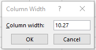
Under Cell Size, click Column Width.
-
In the Column Width box, enter the desired value.
-
Click OK.
To quickly and automatically adjust all columns in a worksheet, click the Select All button, then double-click a border between any two column headers.
-
Modify Workbook Themes in Excel
Modifying a workbook theme means changing the overall look of your worksheet by updating fonts, colors, and the general appearance of objects across all worksheets in the workbook.
To quickly change the fonts, colors, or overall style of objects throughout your workbook, try switching to a different theme or customizing one to suit your needs. If you prefer a specific theme, you can set it as the default for all new workbooks.
Switch to Another Theme
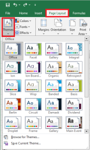
To switch to a different theme, click Page Layout > Themes, then choose the one you want.
Customize a Theme
You can customize a theme by modifying its colors, fonts, and effects to suit your preferences, then save it with the current theme and set it as the default for all new workbooks if desired.
Change Theme Colors
Choosing a different theme color palette or modifying its colors will affect the colors available in the color picker and those already used in your workbook.
-
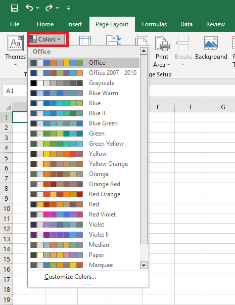
Click Page Layout > Colors, then select your preferred color set.
The first color set is the one used by the current theme.
-
To create your own color set, click Customize Colors.
-
For each theme color to be modified, click the button beneath the color and select one under Theme Colors.
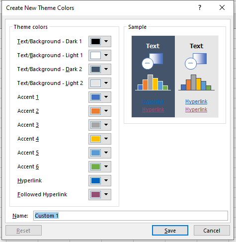
To add your own custom color, click More Colors, then select one from the Standard tab or input values under the Custom tab.
NOTE:
In the Sample area, you get a preview of the changes you have made.-
In the Name field, enter a name for your new color set, then click Save.
NOTE:
You can click Reset before clicking Save if you want to restore the original colors.-
To save these new theme colors with the current theme, go to Page Layout > Themes > Save Current Theme.
Change Theme Fonts
NOTE:
The Preview area shows a preview of your changes.NOTE:
You can click Reset before clicking Save to restore the original colors.Selecting a different theme font lets you update all text at once. For this to work, ensure you’ve used “Headings” and “Body” styles in your formatting.
-
Click Page Layout and select the desired font set.
The first set is used by the current theme.
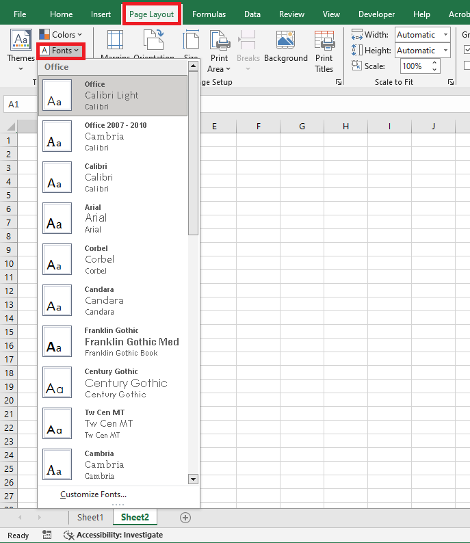
-
To create your own font set, click Customize Fonts.
-
In the Create New Theme Fonts dialog, use the Heading Font and Body Font drop-downs to choose your fonts.
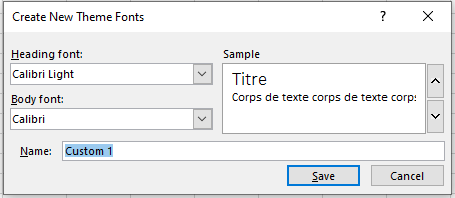
-
In the Name box, enter a name for your custom font set, then click Save.
-
To save these new theme fonts with the current theme, go to Page Layout > Themes > Save Current Theme.
Change Theme Effects
Choosing a different effects set changes the appearance of shapes and objects in your worksheet by applying new borders, shadows, and other visual styles.
-
Click Page Layout and choose your preferred effects set.
The first effects set is used in the current theme.
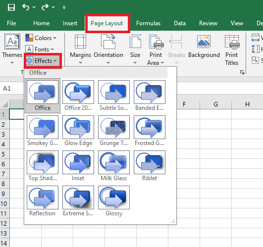
Note: You cannot customize an effects set.
-
To save the selected effects with the current theme, go to Page Layout > Themes > Save Current Theme.
Save a Custom Theme for Reuse
After modifying your theme, you can save it for future use.
-
Go to Page Layout > Themes > Save Current Theme.
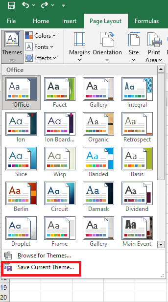
-
In the File Name field, enter a name for your theme, then click Save.
NOTE:
The theme is saved as a theme file (.thmx) in the Document Themes folder on your local drive and is automatically added to the list of custom themes that appear when you click on Themes.Use a Custom Theme as the Default for New Workbooks
To use your custom theme as the default for all new workbooks, apply it to a blank workbook and save it as a template named Book.xltx in the XLStart folder
(typically located at:C:\Users\[username]\AppData\Local\Microsoft\Excel\XLStart).NOTE:
The theme is saved as a.thmxfile in the Document Themes folder on your local drive and is automatically added to the list of custom themes displayed under Themes.Open a Default Theme Automatically
To configure Excel to automatically open a new workbook using Book.xltx:
-
Click File > Options.
-
Under the General tab, in the Startup Options section, uncheck Show the Start screen when this application starts.
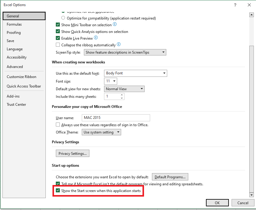
Next time you open Excel, it will launch with the Book.xltx template.
NOTE:
Pressing Ctrl+N also creates a new workbook that uses Book.xltx.-
Inserting and Deleting Columns or Rows in Excel
Inserting a Row or a Column
You can insert a row anywhere in a worksheet as needed. Excel shifts the existing rows downward to make room for the new one.
To insert a row:
-
Click anywhere in the row below where you want the new row to appear.
-
Select Insert Rows from the menu bar.

A new row is inserted above the originally selected cell(s).
Alternatively:
-
Click anywhere in the row below where you want the new row.
-
Right-click and choose Insert from the context menu.

The Insert dialog box appears.
-
Choose Entire Row.
-
Click OK.
A new row is inserted above the originally selected cell(s).

To insert multiple rows, select the same number of rows before choosing Insert. Excel inserts the same number of new rows as you originally selected.
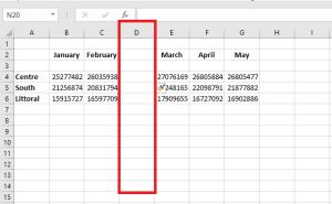
You can also insert a column anywhere in a worksheet. Excel shifts the existing columns to the right to make space for the new one.
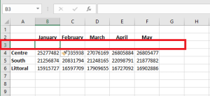
To insert a column:
-
Click anywhere in the column where you want to insert a new column.
-
Choose Insert Columns from the menu bar.
A new column is inserted to the left of the existing column.
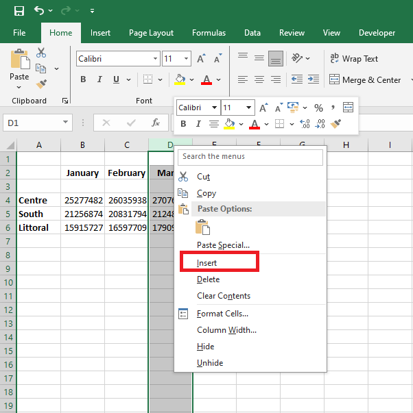
Alternatively:
-
Click anywhere in the column where you want to insert the new column.
-
Right-click and choose Insert from the context menu.
The Insert dialog box appears.
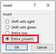
-
Click Entire Column in the Insert dialog box.
-
Click OK.
A new column is inserted to the left of the existing column.
You can also select multiple columns before choosing Insert to quickly add multiple columns. Excel inserts the same number of new columns as originally selected.
Deleting Columns and Rows
Deleting columns and rows works the same way as inserting them.
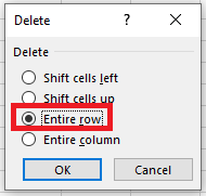
To delete a row and all its contents:
-
Select a cell in the row to delete.
-
Choose Edit > Delete from the menu bar.
-
In the Delete dialog box, click Entire Row.
-
Click OK.
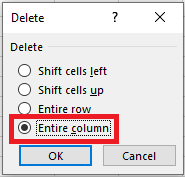
To delete a column and all its contents:
-
Select a cell in the column to delete.
-
Choose Edit > Delete from the menu bar.
-
In the Delete dialog box, click Entire Column.
-
Click OK.
-
Modify the Page Layout in Excel
You may often find yourself in a situation where you need to print the Excel sheet containing important data to be shared in hard copy. In such cases, page layout becomes essential. Once you learn how to handle this in Microsoft Excel, printing pages becomes easier. Several operations are involved in setting up the page, such as:
-
Adjusting the margins for top, bottom, left, and right
-
Adding a header or footer to the Excel sheet you want to print
-
Page views: Portrait, Landscape, or Custom
-
Setting the print area, etc.
We will review all the page setup settings and options one by one in this section. It’s very easy in Excel to configure the page before printing and preview it to make adjustments as needed.
Page Layout Using the View Tab
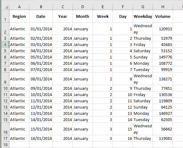
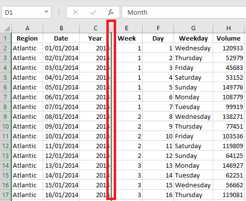
Let’s suppose we have data as shown below.

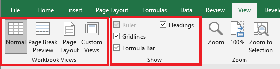
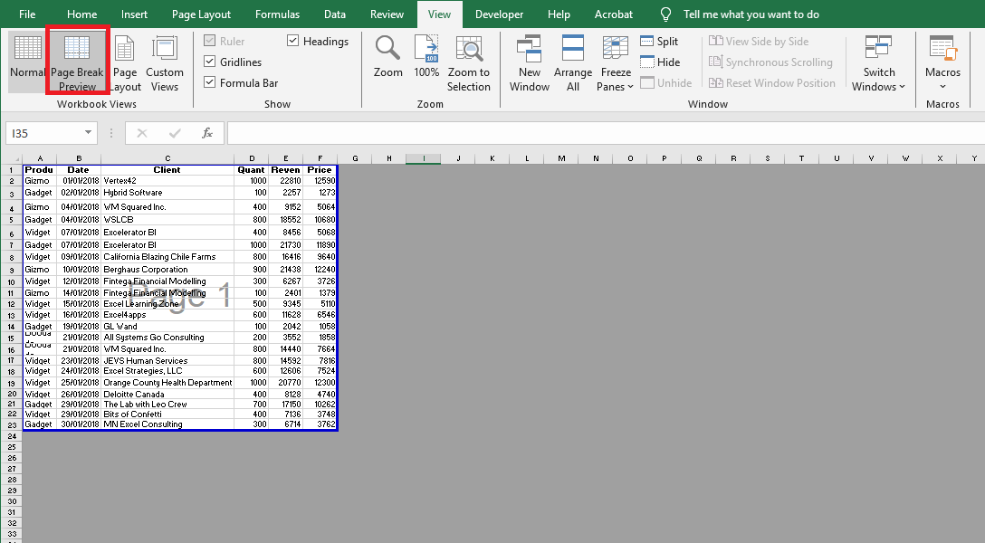
Click on the View tab in the Excel ribbon at the top of your sheet. You will see several options under two groups: Workbook Views and Show. Under Workbook Views, you will find different types of views: Normal view, Page Break Preview, Page Layout, Custom Views.
Click Page Break Preview. It will split your page based on the print area, as shown below.
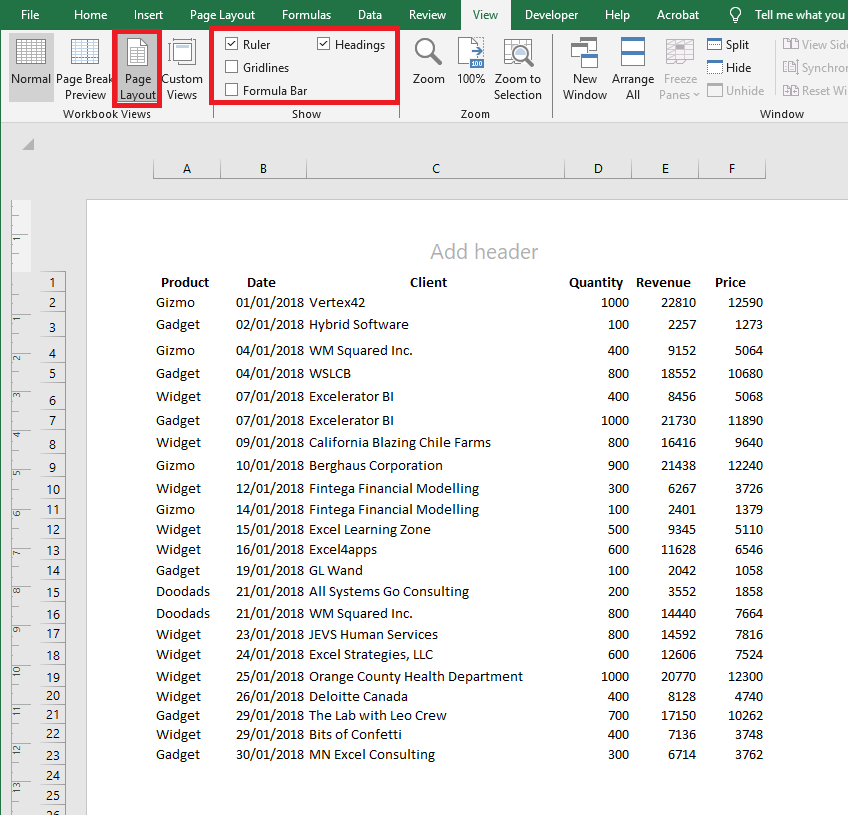
Click the Page Layout option to see the Excel sheet in layout format. It already shows the default header, and you can add « Sales Data for the Year 2018 » as a title. Under the Show option, you can check or uncheck various options such as ruler, gridlines, etc.
Setting Margins
Sometimes, the columns on your print page take up the entire width, and one column still doesn’t fit, causing it to be printed on the next page. To solve this, we can use the Margins option under the Page Layout tab in Excel.
Click the Page Layout tab in Excel. You’ll see a variety of commands, each with several options.
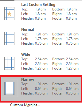
Under Page Setup, click the Margins button. You’ll see different margin presets: Custom, Normal, Wide, and Narrow. Choose the one that best suits your needs.

Click Narrow Margins to tighten the space and fit more columns on one page.
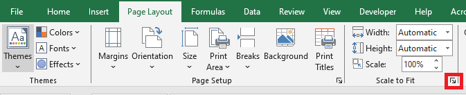
You can also use the Page Setup dialog box to configure margin settings.
Click the Page Layout tab, then in the Page Setup group, click the Dialog Box Launcher.
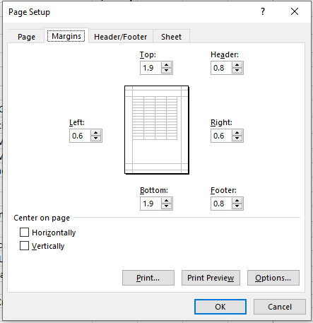
Enter the margin settings and preview the results in the Preview area:
-
Top, Bottom, Left, Right: Adjust the values to specify the distance between your data and the edges of the printed page.
-
Header or Footer: Enter a value to adjust the distance between the header/footer and the top/bottom of the page. This must be smaller than the margin to prevent overlap.
-
Center on Page: Center your data on the page horizontally, vertically, or both by checking the appropriate boxes.
Page Orientation in Page Layout
Sometimes adjusting margins isn’t enough to fit all your columns on one page. In that case, you may need to change the page orientation.
Go to the Page Layout tab and select the Orientation button next to Margins.
Clicking Orientation will show two options: Portrait and Landscape.
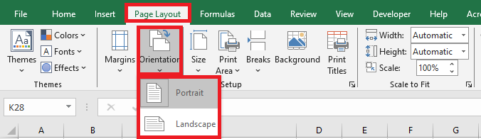
By default, orientation is set to Portrait. Change it to Landscape to ensure all columns are visible on one printed page.
Adjusting Page Size in Page Layout
You can also modify the paper size for a proper printout. Go to the Page Layout tab and click the Size button. This lets you choose the paper size for your printed document.
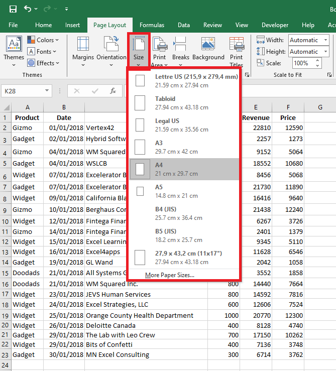
A list of paper sizes will appear, such as Letter, Legal, A4, A3, etc. By default, it may be set to Letter (especially after changing the orientation to Landscape).
Click A4 to set the page size to A4, which is the most commonly used paper format.
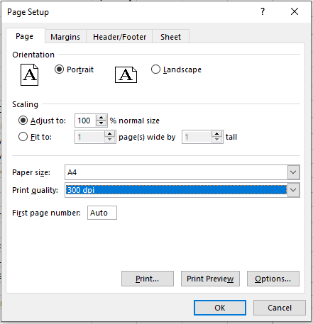
You can also use the Page Setup dialog box to configure the Page tab options.
Click the Page Layout tab, then click the Dialog Box Launcher in the Page Setup group.
-
Orientation: Choose between Portrait and Landscape.
-
Scaling: Enlarges or reduces the worksheet or selection to fit the specified number of pages when printed.
-
Adjust to: Enter a percentage to scale the worksheet.
-
Fit to: Enter a number of pages wide and/or tall. To fill the page width and use as many pages as needed vertically, type 1 for pages wide and leave the height blank.
-
-
Paper Size: Choose Letter, Legal, or another format depending on what you want for your printed document.
-
Print Quality: Choose a resolution (DPI – dots per inch). Higher resolution provides better print quality if supported by the printer.
-
First Page Number: Enter « Auto » to start numbering at 1, or enter a different number to start from another page number.
Print Titles in Page Layout
If your data is long—say, 10,000 rows—it will certainly span multiple pages. The problem is that column headers are only printed on the first page. For subsequent pages, it becomes hard to know which column is which. Printing column titles on each page is essential.
Click the Page Layout tab and then the Print Titles button.
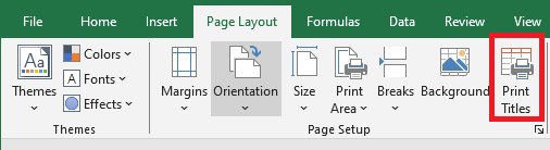
Clicking Print Titles opens the Page Setup window with the Sheet tab active.
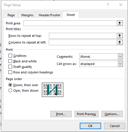
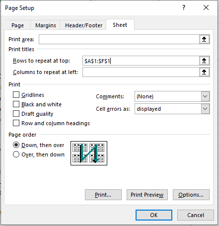
Under this tab, click the Rows to repeat at top field. This lets you specify which rows will be printed at the top of every page. For example:
$A$1:$F$1.You can also set the Print Area, Columns to repeat at left, and more in this Sheet tab. Click OK once you’re done.
Summary and Things to Remember
-
Print Area: Click inside the Print Area field, then drag to select the range you want to print. The collapse dialog button helps you shrink the dialog to select from the worksheet. Click it again to return to the full dialog.
-
Print Titles:
-
Use Rows to repeat at top for horizontal titles.
-
Use Columns to repeat at left for vertical titles.
Then select the relevant cells in your worksheet.
-
-
Print Settings:
-
Gridlines: Check this box to print gridlines. They are not printed by default.
-
Black and White: Use this if your printer is color-capable but you want black and white output.
-
Draft Quality: Enables faster, lower-quality printing if supported by your printer.
-
Row and Column Headings: Include these in the printout by checking the box.
-
Comments and Notes:
-
At end of sheet: Print all notes on a summary page.
-
As displayed on sheet: Print notes where they appear on the sheet.
-
None: Default setting; comments are not printed.
-
-
-
Cell Errors As: Choose how to display errors in printouts:
-
As displayed (default)
-
<blank>
-
—
-
#N/A
-
-
Page Order: Choose Down, then over or Over, then down to set how Excel numbers and prints pages. A preview image shows the order.
-