Votre panier est actuellement vide !
Étiquette : vba
Implement Advanced Data Visualization Techniques with Excel VBA
In Excel, data visualization helps users interpret and present data more effectively. While Excel’s built-in charts and graphs provide basic functionality, VBA can enhance this with advanced techniques that allow for dynamic and interactive visualizations.
Some advanced data visualization techniques include:
- Dynamic Charting (charts that update automatically based on changes in data)
- Conditional Formatting (using color gradients, data bars, and icons to visually highlight patterns in data)
- Combo Charts (combining different types of charts like line and column in one chart)
- Dynamic Dashboard (interactive, visually appealing reports with multiple charts and controls)
Step-by-Step VBA Implementation for Advanced Visualizations
Let’s dive into the code and techniques. The examples provided will be designed for specific purposes, such as creating dynamic charts and using conditional formatting.
- Dynamic Charting
Dynamic charts automatically update when the data changes. Let’s say you have a dataset with sales data for each month, and you want the chart to adjust automatically whenever new data is added.
VBA Code for Dynamic Charting
Sub CreateDynamicChart()
    Dim ws As Worksheet
    Dim chartObject As ChartObject
    Dim dataRange As Range
    Dim chartRange As Range
    ' Set reference to the worksheet
    Set ws = ThisWorkbook.Sheets("SalesData")
    ' Define the data range dynamically
    ' Assuming data is in columns A and B, starting from row 1
    Set dataRange = ws.Range("A1:B" & ws.Cells(ws.Rows.Count, "A").End(xlUp).Row)
    ' Create a chart
    Set chartObject = ws.ChartObjects.Add(Left:=100, Width:=375, Top:=75, Height:=225)
    ' Define chart range for dynamic data
    chartObject.Chart.SetSourceData Source:=dataRange
    ' Set chart type (line chart in this case)
    chartObject.Chart.ChartType = xlLine
    ' Adding a title
    chartObject.Chart.HasTitle = True
    chartObject.Chart.ChartTitle.Text = "Sales Trend"
    ' Customize the chart
    chartObject.Chart.Axes(xlCategory, xlPrimary).HasTitle = True
    chartObject.Chart.Axes(xlCategory, xlPrimary).AxisTitle.Text = "Month"
    chartObject.Chart.Axes(xlValue, xlPrimary).HasTitle = True
    chartObject.Chart.Axes(xlValue, xlPrimary).AxisTitle.Text = "Sales"
End Sub
Explanation
- Dynamic Range: The data range is dynamically defined based on the last non-empty row in column A. The code automatically adjusts to include all rows with data.
- Chart Creation: The code creates a line chart based on the dynamic range and applies some formatting (like titles and axis labels).
- Conditional Formatting
Conditional formatting allows you to apply visual elements (such as colors or icons) to cells based on the value. For example, you might want to highlight sales figures above a certain threshold in green and those below in red.
VBA Code for Conditional Formatting
Sub ApplyConditionalFormatting()
    Dim ws As Worksheet
    Dim dataRange As Range
    ' Set reference to the worksheet
    Set ws = ThisWorkbook.Sheets("SalesData")
    ' Define the range to apply formatting (Assuming sales data in column B)
    Set dataRange = ws.Range("B2:B" & ws.Cells(ws.Rows.Count, "B").End(xlUp).Row)
    ' Clear any existing formatting
    dataRange.FormatConditions.Delete
    ' Apply conditional formatting (Green for sales > 1000, Red for sales < 500)
    With dataRange.FormatConditions.Add(Type:=xlCellValue, Operator:=xlGreater, Formula1:="1000")
        .Interior.Color = RGB(0, 255, 0) ' Green color for sales > 1000
    End With
    With dataRange.FormatConditions.Add(Type:=xlCellValue, Operator:=xlLess, Formula1:="500")
        .Interior.Color = RGB(255, 0, 0) ' Red color for sales < 500
    End With
End Sub
Explanation
- FormatConditions: This object allows you to apply conditional formatting. We used xlCellValue to format based on the cell’s value.
- Color Coding: Green is applied to cells with values greater than 1000, while red is applied to cells with values less than 500.
- Combo Charts
A combo chart combines different chart types (such as a column chart for one data series and a line chart for another). This is useful when you want to display different data trends on the same graph (e.g., showing sales revenue as columns and profit margins as a line).
VBA Code for Combo Chart
Sub CreateComboChart()
    Dim ws As Worksheet
    Dim chartObject As ChartObject
    Dim dataRange As Range
    ' Set reference to the worksheet
    Set ws = ThisWorkbook.Sheets("SalesData")
    ' Define the data range (Assuming data in columns A, B, and C)
    Set dataRange = ws.Range("A1:C" & ws.Cells(ws.Rows.Count, "A").End(xlUp).Row)
    ' Create a chart
    Set chartObject = ws.ChartObjects.Add(Left:=100, Width:=500, Top:=100, Height:=300)
    ' Set source data
    chartObject.Chart.SetSourceData Source:=dataRange
    ' Create combo chart (columns for data 2, line for data 3)
    chartObject.Chart.ChartType = xlColumnClustered
    chartObject.Chart.SeriesCollection(1).ChartType = xlColumnClustered ' Column for sales
    chartObject.Chart.SeriesCollection(2).ChartType = xlLine ' Line for profit margin
    ' Add titles
    chartObject.Chart.HasTitle = True
    chartObject.Chart.ChartTitle.Text = "Sales and Profit Margin"
    chartObject.Chart.Axes(xlCategory, xlPrimary).AxisTitle.Text = "Month"
    chartObject.Chart.Axes(xlValue, xlPrimary).AxisTitle.Text = "Sales"
End Sub
Explanation
- Chart Types: The first series (e.g., sales) is displayed as columns, while the second series (e.g., profit margin) is displayed as a line.
- Combo Charts: Excel allows you to mix different chart types to enhance data visualization.
- Dynamic Dashboard
A dynamic dashboard is an interactive report where users can filter data or select certain elements to see related visuals. This is a more complex feature, but VBA can help automate and control this.
Basic Example: Adding a Button to Update a Chart
Here’s a simple implementation that allows a button click to change a chart’s data range dynamically.
Sub CreateDashboard()
    Dim ws As Worksheet
    Dim button As Object
    Dim chartObject As ChartObject
    ' Set reference to the worksheet
    Set ws = ThisWorkbook.Sheets("Dashboard")
    ' Add a button
    Set button = ws.Buttons.Add(Left:=100, Top:=50, Width:=100, Height:=30)
    button.Caption = "Update Chart"
    ' Assign a macro to update the chart when the button is clicked
    button.OnAction = "UpdateChart"
    ' Add a chart
    Set chartObject = ws.ChartObjects.Add(Left:=100, Top:=100, Width:=375, Height:=225)
    chartObject.Chart.ChartType = xlColumnClustered
    chartObject.Chart.HasTitle = True
    chartObject.Chart.ChartTitle.Text = "Sales Overview"
End Sub

Sub UpdateChart()
    Dim ws As Worksheet
    Dim chartObject As ChartObject
    Dim newRange As Range
    ' Set reference to the worksheet
    Set ws = ThisWorkbook.Sheets("Dashboard")
    ' Update the chart with a new data range
    Set chartObject = ws.ChartObjects(1)
    Set newRange = ws.Range("A1:B10") ' New dynamic range for chart
    chartObject.Chart.SetSourceData Source:=newRange
End Sub
Explanation
- Button Control: The button triggers the UpdateChart subroutine, which updates the chart’s data range.
- Dynamic Chart Update: The UpdateChart subroutine changes the source data for the chart when the button is pressed.
Conclusion
Using VBA in Excel, you can significantly enhance your data visualization capabilities. The examples provided cover dynamic charts, conditional formatting, combo charts, and even dashboard interactivity. You can extend these techniques by incorporating more advanced concepts like pivot charts, advanced filtering, or integrating with external data sources.
Implement Advanced Data Validation Techniques with Excel VBA
Objective:
We will create a VBA code that implements complex data validation techniques such as:
- Custom Validation Lists that are dynamic and depend on other cell values.
- Date Range Validation ensuring data falls within a specific date range.
- Text Length Validation to restrict the number of characters entered in a cell.
- Formula-based Validation that validates based on a custom formula.
Step-by-Step VBA Code Example
Sub ImplementAdvancedDataValidation()
    Dim ws As Worksheet
    Dim rng As Range
    ' Set the target worksheet and the range where validation will be applied
    Set ws = ThisWorkbook.Sheets("Sheet1")
    ' Example 1: Custom Dynamic List Validation
    ' The validation will depend on the value of cell A1
    ' If A1 is "Fruits", the list should contain "Apple", "Banana", "Orange"
    ' If A1 is "Vegetables", the list should contain "Carrot", "Potato", "Tomato"
    Set rng = ws.Range("B2:B10") ' Range where validation will be applied
    ' Clear existing validations
    rng.Validation.Delete
    ' Add a dynamic validation list
    If ws.Range("A1").Value = "Fruits" Then
        rng.Validation.Add Type:=xlValidateList, AlertStyle:=xlValidAlertStop, _
                           Operator:=xlBetween, Formula1:="Apple,Banana,Orange"
    ElseIf ws.Range("A1").Value = "Vegetables" Then
        rng.Validation.Add Type:=xlValidateList, AlertStyle:=xlValidAlertStop, _
                           Operator:=xlBetween, Formula1:="Carrot,Potato,Tomato"
    End If
    rng.Validation.IgnoreBlank = True
    rng.Validation.InCellDropdown = True
    ' Example 2: Date Range Validation
    ' Ensures the entered date is between 01-Jan-2020 and 31-Dec-2025
    Set rng = ws.Range("C2:C10")
    ' Clear existing validations
    rng.Validation.Delete
    ' Add date range validation
    rng.Validation.Add Type:=xlValidateDate, AlertStyle:=xlValidAlertStop, _
                       Operator:=xlBetween, Formula1:="01/01/2020", Formula2:="31/12/2025"
    rng.Validation.IgnoreBlank = True
    rng.Validation.InCellDropdown = False
    ' Example 3: Text Length Validation
    ' Restrict text length to be between 5 and 15 characters
    Set rng = ws.Range("D2:D10")
    ' Clear existing validations
    rng.Validation.Delete
    ' Add text length validation
    rng.Validation.Add Type:=xlValidateTextLength, AlertStyle:=xlValidAlertStop, _
                       Operator:=xlBetween, Formula1:=5, Formula2:=15
    rng.Validation.IgnoreBlank = True
    rng.Validation.InCellDropdown = False
    ' Example 4: Formula-based Validation
    ' Ensure that the value in E2:E10 is greater than the value in D2:D10
    Set rng = ws.Range("E2:E10")
    ' Clear existing validations
    rng.Validation.Delete
    ' Add formula-based validation
    rng.Validation.Add Type:=xlValidateCustom, AlertStyle:=xlValidAlertStop, _
                       Operator:=xlBetween, Formula1:="=E2>D2"
    rng.Validation.IgnoreBlank = True
    rng.Validation.InCellDropdown = False
    ' Final Message
    MsgBox "Advanced Data Validation has been applied successfully!", vbInformation
End Sub
Detailed Explanation of Each Step
- Dynamic List Validation Based on Another Cell’s Value (Example 1)
‘ Create a dynamic validation list based on the value of cell A1
If ws.Range("A1").Value = "Fruits" Then rng.Validation.Add Type:=xlValidateList, Formula1:="Apple,Banana,Orange" ElseIf ws.Range("A1").Value = "Vegetables" Then rng.Validation.Add Type:=xlValidateList, Formula1:="Carrot,Potato,Tomato" End If- Goal: This technique allows you to create a dependent dropdown list. The list options change depending on the value entered in a parent cell (e.g., A1).
- How it works:
- The Validation.Add method applies data validation to a specified range.
- If cell A1 contains « Fruits, » the dropdown in B2:B10 will show fruit options. If A1 contains « Vegetables, » the dropdown will show vegetable options.
- Date Range Validation (Example 2)
' Validate that entered date is between 01-Jan-2020 and 31-Dec-2025
rng.Validation.Add Type:=xlValidateDate, Formula1:="01/01/2020", Formula2:="31/12/2025"
- Goal: This ensures that the data entered is a valid date within a specific date range.
- How it works:
- The xlValidateDate validation type is used.
- Formula1 and Formula2 specify the start and end dates of the valid range.
- If the user enters a date outside this range, Excel will trigger an error message.
- Text Length Validation (Example 3)
' Validate that the entered text length is between 5 and 15 characters
rng.Validation.Add Type:=xlValidateTextLength, Formula1:=5, Formula2:=15
- Goal: This limits the length of text input in cells to a specific range, preventing excessively short or long entries.
- How it works:
- The xlValidateTextLength type is used to restrict text input to a range defined by Formula1 (minimum characters) and Formula2 (maximum characters).
- Users can only enter text that is between 5 and 15 characters in length.
- Formula-based Validation (Example 4)
' Ensure the value in E2:E10 is greater than the value in D2:D10
rng.Validation.Add Type:=xlValidateCustom, Formula1:="=E2>D2"
- Goal: This validation uses a custom formula to compare values between two columns, ensuring one is greater than the other.
- How it works:
- The xlValidateCustom validation type allows the use of an Excel formula for validation.
- The formula « =E2>D2 » checks that the value in column E is greater than the value in column D. If the condition is not met, the user will see an error message.
Additional Features:
- Error Messages: You can customize the error message using ErrorTitle and ErrorMessage properties in the Validation object.
- Data Entry Handling: By setting the InCellDropdown property to True, you ensure the user can see a dropdown for list-based validations.
- Clearing Validations: The Validation.Delete method is used to clear any existing validations before applying new ones.
Conclusion
By using the techniques above, you can create robust data validation rules in Excel through VBA. This allows for dynamic, formula-based, and even context-sensitive validation rules, ensuring the data entered into your Excel worksheets adheres to your specific requirements.
Implement Advanced Data TransFormation Techniques with Excel VBA
Scenario
Let’s imagine you have a dataset with multiple columns, and you want to transform it into a more useful format. For example, you might need to:
- Pivot a table of data (turn rows into columns).
- Unpivot data (turn columns into rows).
- Clean data by removing unwanted characters or handling missing values.
- Apply complex filters or transform the data based on certain criteria.
I will break down the techniques and provide a VBA code example for each one.
- Pivoting Data (Turning Rows into Columns)
Problem: You have a list of sales data for multiple sales representatives across different months, but the data is in rows, and you want to pivot it so that each month becomes a separate column.
Example Data:
Sales Rep Month Sales Amount Alice Jan 200 Alice Feb 250 Bob Jan 300 Bob Feb 400 Desired Output:
Sales Rep Jan Feb Alice 200 250 Bob 300 400 VBA Code for Pivoting Data:
Sub PivotData()
    Dim ws As Worksheet
    Dim lastRow As Long, lastCol As Long
    Dim dataRange As Range
    Dim pivotTable As PivotTable
    Dim pivotCache As PivotCache
    ' Set the worksheet and range
    Set ws = ThisWorkbook.Sheets("Sheet1")
    lastRow = ws.Cells(ws.Rows.Count, 1).End(xlUp).Row
    lastCol = ws.Cells(1, ws.Columns.Count).End(xlToLeft).Column
    Set dataRange = ws.Range(ws.Cells(1, 1), ws.Cells(lastRow, lastCol))
    ' Create a Pivot Cache
    Set pivotCache = ThisWorkbook.PivotTableWizard(dataRange)
    ' Create the Pivot Table on a new sheet
    Set wsPivot = ThisWorkbook.Sheets.Add
    Set pivotTable = wsPivot.PivotTableWizard(pivotCache, _
                                              ws.Cells(1, 1), _
                                              ws.Cells(1, 2), _
                                              ws.Cells(1, 3))
    ' Organize Pivot Table Fields
    pivotTable.PivotFields("Sales Rep").Orientation = xlRowField
    pivotTable.PivotFields("Month").Orientation = xlColumnField
    pivotTable.PivotFields("Sales Amount").Orientation = xlDataField
    pivotTable.PivotFields("Sales Amount").Function = xlSum
End Sub
Explanation:
- We define the data range that contains the dataset.
- Create a pivot cache and then use the PivotTableWizard method to create a new pivot table on a separate sheet.
- Set the field orientation for rows (Sales Rep), columns (Month), and data (Sales Amount) to display the sum of sales.
- Unpivoting Data (Turning Columns into Rows)
Problem: You have a wide dataset, and you want to transform it into a long format (unpivot the data).
Example Data:
Sales Rep Jan Feb Alice 200 250 Bob 300 400 Desired Output:
Sales Rep Month Sales Amount Alice Jan 200 Alice Feb 250 Bob Jan 300 Bob Feb 400 VBA Code for Unpivoting Data:
Sub UnpivotData()
    Dim ws As Worksheet
    Dim lastRow As Long, lastCol As Long
    Dim i As Long, j As Long
    Dim targetRow As Long
    Dim monthName As String
    Dim salesAmount As Double
    ' Set worksheet reference
    Set ws = ThisWorkbook.Sheets("Sheet1")
    lastRow = ws.Cells(ws.Rows.Count, 1).End(xlUp).Row
    lastCol = ws.Cells(1, ws.Columns.Count).End(xlToLeft).Column
    ' Start populating the new unpivoted data below the existing data
    targetRow = lastRow + 2
    ' Write headers for unpivoted data
    ws.Cells(targetRow, 1).Value = "Sales Rep"
    ws.Cells(targetRow, 2).Value = "Month"
    ws.Cells(targetRow, 3).Value = "Sales Amount"
    targetRow = targetRow + 1
    ' Loop through the data to unpivot
    For i = 2 To lastRow
        For j = 2 To lastCol
            monthName = ws.Cells(1, j).Value
            salesAmount = ws.Cells(i, j).Value
            ws.Cells(targetRow, 1).Value = ws.Cells(i, 1).Value ' Sales Rep
            ws.Cells(targetRow, 2).Value = monthName ' Month
            ws.Cells(targetRow, 3).Value = salesAmount ' Sales Amount
            targetRow = targetRow + 1
        Next j
    Next i
End Sub
Explanation:
- We loop through each row and column of the original dataset.
- For each combination of Sales Rep and Month, we create a new row in the output table with the corresponding month and sales amount.
- The data is now in a long format, suitable for analysis or further transformations.
- Cleaning Data (Removing Unwanted Characters)
Problem: Your dataset contains unwanted spaces or special characters, and you want to clean the data.
Example Data:
Name Age Address John Doe 30 123 Main St. Alice@! 25 456 Elm St.#$ VBA Code for Cleaning Data:
Sub CleanData()
    Dim ws As Worksheet
    Dim lastRow As Long
    Dim i As Long
    Dim cell As Range
    ' Set worksheet reference
    Set ws = ThisWorkbook.Sheets("Sheet1")
    lastRow = ws.Cells(ws.Rows.Count, 1).End(xlUp).Row
    ' Loop through each row to clean data
    For i = 2 To lastRow
        ' Clean Name - Remove special characters and extra spaces
        Set cell = ws.Cells(i, 1)
        cell.Value = Trim(Replace(cell.Value, "@", ""))
        cell.Value = Trim(Replace(cell.Value, "!", ""))
        ' Clean Address - Remove special characters
        Set cell = ws.Cells(i, 3)
        cell.Value = Trim(Replace(cell.Value, "#", ""))
    Next i
End Sub
Explanation:
- We loop through the rows and clean up the unwanted characters (like @, !, #, etc.) and extra spaces in the Name and Address columns.
- The Trim() function removes leading and trailing spaces, and the Replace() function is used to replace unwanted characters.
- Complex Filtering (Applying Multiple Criteria)
Problem: You need to filter a dataset based on multiple conditions (e.g., sales greater than a certain value and from a specific region).
Example Data:
Sales Rep Region Sales Amount Alice North 200 Bob South 300 Alice South 150 John North 500 VBA Code for Complex Filtering:
Sub FilterData()
    Dim ws As Worksheet
    Dim lastRow As Long
    Dim i As Long
    Dim salesAmount As Double
    Dim region As String
    ' Set worksheet reference
    Set ws = ThisWorkbook.Sheets("Sheet1")
    lastRow = ws.Cells(ws.Rows.Count, 1).End(xlUp).Row
    ' Loop through each row to apply the filter criteria
    For i = 2 To lastRow
        salesAmount = ws.Cells(i, 3).Value
        region = ws.Cells(i, 2).Value
        ' Only keep rows where Sales Amount > 200 and Region is North
        If salesAmount > 200 And region = "North" Then
            ws.Rows(i).Hidden = False
        Else
            ws.Rows(i).Hidden = True
        End If
    Next i
End Sub
Explanation:
- We loop through the dataset and apply a filter where the Sales Amount is greater than 200, and the Region is « North. »
- Rows that do not meet these criteria are hidden.
Conclusion
These are just a few of the advanced data transformation techniques you can implement using VBA in Excel. With these methods, you can pivot and unpivot your data, clean it, and apply complex filters to make your dataset more useful for analysis. VBA allows you to automate these tasks, saving you time and ensuring consistency.
Implement Advanced Data TransFormation Pipelines with Excel VBA
Implementing an advanced data transformation pipeline using Excel VBA involves various steps like cleaning data, performing calculations, aggregating, transforming, and finally loading it into a desired format. Here’s a detailed VBA code with step-by-step explanations:
Scenario
We will create a pipeline that performs the following operations on data:
- Data Loading: Import raw data from a worksheet.
- Data Cleaning: Remove empty rows, handle missing values, and standardize text.
- Data Transformation: Perform some mathematical operations or aggregations.
- Data Output: Output the transformed data to a new worksheet.
Structure of the VBA Code
Sub AdvancedDataTransformationPipeline()

    ' Declare Variables

    Dim wsSource As Worksheet

    Dim wsOutput As Worksheet

    Dim lastRow As Long
    Dim i As Long
    Dim value As Double
    Dim cleanData As Collection
    Dim cleanedRow As Variant
    Dim rowCount As Long
    ' Set worksheets
    Set wsSource = ThisWorkbook.Sheets("RawData") ' Raw Data worksheet
    Set wsOutput = ThisWorkbook.Sheets("CleanedData") ' Output worksheet
    ' Get the last row with data in the source sheet
    lastRow = wsSource.Cells(wsSource.Rows.Count, "A").End(xlUp).Row
    ' Clear existing data in the Output sheet
    wsOutput.Cells.Clear
    ' Step 1: Data Cleaning
    Set cleanData = New Collection
    For i = 2 To lastRow ' Assuming row 1 is headers
        ' Read the data row by row
        cleanedRow = Application.Transpose(wsSource.Range("A" & i & ":D" & i).Value)
        ' Step 1.1: Remove rows with empty values
        If Not IsEmpty(cleanedRow(1)) And Not IsEmpty(cleanedRow(2)) Then
            ' Step 1.2: Handle missing values (replace empty cells with default value 0)
            For j = 1 To UBound(cleanedRow)
                If IsEmpty(cleanedRow(j)) Then
                    cleanedRow(j) = 0 ' Default value for missing data
                End If
            Next j
            ' Step 1.3: Standardize text (trim spaces, capitalize)
            cleanedRow(3) = Trim(UCase(cleanedRow(3))) ' Assuming column C has the text to standardize
            ' Add the cleaned data row to the collection
            cleanData.Add cleanedRow
        End If
    Next i
    ' Step 2: Data Transformation
    rowCount = 1 ' Starting row for output
    For Each cleanedRow In cleanData
        ' Write the cleaned data to the output worksheet
        wsOutput.Cells(rowCount, 1).Value = cleanedRow(1)
        wsOutput.Cells(rowCount, 2).Value = cleanedRow(2)
        wsOutput.Cells(rowCount, 3).Value = cleanedRow(3)
        ' Step 2.1: Perform transformation (example: apply a formula or calculation)
        value = cleanedRow(2) * 1.1 ' Example: apply a 10% increase to the second column's value
        wsOutput.Cells(rowCount, 4).Value = value
        rowCount = rowCount + 1
    Next cleanedRow
    ' Step 3: Aggregation (optional)
    ' For example, sum the transformed column
    Dim total As Double
    total = 0
    For i = 2 To rowCount - 1
        total = total + wsOutput.Cells(i, 4).Value
    Next i
    ' Write total in the next available row
    wsOutput.Cells(rowCount, 4).Value = "Total"
    wsOutput.Cells(rowCount, 5).Value = total
    MsgBox "Data transformation complete!"
End Sub
Step-by-Step Explanation
- Declare Variables: We begin by declaring variables for the source and output worksheets, as well as for the last row of data, loop counters, and a collection to store cleaned data.
- Set Worksheets:
- wsSource is the worksheet that contains the raw data, named « RawData ».
- wsOutput is the worksheet where the transformed data will be written, named « CleanedData ».
- Data Cleaning Loop:
- We loop through the rows in the wsSource worksheet starting from row 2 (assuming row 1 contains headers).
- For each row, we:
- Remove rows with empty values: If either the first or second cell is empty, that row is skipped.
- Handle missing values: If any cell in the row is empty, it is replaced with a default value (0 in this case).
- Standardize text: If the third column contains text, it is trimmed (extra spaces are removed) and capitalized (converted to uppercase).
- Data Transformation:
- After cleaning, the data is stored in a collection (cleanData).
- We then loop through the collection, and for each cleaned row, we:
- Write the cleaned values to the wsOutput worksheet.
- Apply a transformation: In this example, the second column’s value is increased by 10%. You can replace this calculation with your own transformation logic.
- Aggregation:
- After the transformed data is written, we aggregate the data. In this case, we sum up the values in the fourth column (which contains the transformed data) and display the total in the next row.
- This step is optional and can be customized for other types of aggregation like average, count, etc.
- Completion Message: After all the steps are done, a message box is displayed to let the user know that the data transformation is complete.
How to Use
- Prepare your workbook: Ensure that your raw data is in the « RawData » worksheet. The columns should be consistent with the data structure defined in the code (for example, four columns: one with numeric values, one with text, etc.).
- Run the Macro: Open the VBA editor (Alt + F11), paste the code into a new module, and then run it (F5). The cleaned and transformed data will be output to the « CleanedData » worksheet.
Customization
- Column Structure: If your data structure is different, you can change the range of columns and rows accordingly.
- Transformation Logic: The code currently applies a 10% increase to the numeric data in the second column. You can modify this logic to perform any other transformation or calculation.
- Aggregation: You can add other aggregation logic like calculating the average or counting certain values depending on your requirements.
This is a robust starting point for implementing an advanced data transformation pipeline using Excel VBA.
Implement Advanced Data TransFormation Functions
I will walk you through several key concepts like data cleaning, transformation, and manipulation using VBA, with long and detailed explanations.
- Context
In Excel, we often need to work with large datasets, perform various transformations (like converting, cleaning, or filtering data), and create dynamic reports. Excel VBA is a powerful tool for automating these tasks. Advanced data transformation might involve actions like:
- Removing duplicates based on certain conditions.
- Reorganizing data into different formats (pivoting/unpivoting).
- Grouping and aggregating data.
- Handling missing data (like filling in blanks).
- Merging multiple datasets based on common keys.
In the following code, I’ll demonstrate a few of these transformations. I’ll add detailed comments to explain every part of the code.
2. Removing Duplicates with Specific Conditions
Let’s start with a common transformation: removing duplicates based on certain criteria.
Sub RemoveDuplicatesAdvanced()
    ' Define variables
    Dim ws As Worksheet
    Dim dataRange As Range
    Dim uniqueColumns As Variant
    ' Set the worksheet object to the active sheet
    Set ws = ThisWorkbook.Sheets("Sheet1")
    ' Define the range of data (assuming data starts from A1 and ends at the last row in column A)
    Set dataRange = ws.Range("A1").CurrentRegion
    ' Define which columns to consider for finding duplicates (e.g., columns 1 and 2)
    uniqueColumns = Array(1, 2) ' Check duplicates based on Column A and B
    ' Remove duplicates
    dataRange.RemoveDuplicates Columns:=uniqueColumns, Header:=xlYes
    MsgBox "Duplicates removed successfully!"
End Sub
Explanation:
- Define Variables:
- ws: Refers to the worksheet where the data is.
- dataRange: Refers to the range of data where we want to perform the operation.
- uniqueColumns: Specifies the columns that will be used to detect duplicates (e.g., Column A and Column B).
- Set the Range: The CurrentRegion property automatically detects the range of data, expanding to include all adjacent non-empty cells.
- Remove Duplicates: The RemoveDuplicates method removes rows where the values in the specified columns are identical.
- Grouping and Aggregating Data (Summing Values by Group)
Sometimes, you need to group data by a certain column and perform an aggregation like summing the values in another column.
Sub GroupAndAggregateData()
    ' Define variables
    Dim ws As Worksheet
    Dim lastRow As Long
    Dim dataRange As Range
    Dim resultRange As Range
    Dim dict As Object
    Dim i As Long
    ' Set worksheet and get the last row
    Set ws = ThisWorkbook.Sheets("Sheet1")
    lastRow = ws.Cells(ws.Rows.Count, "A").End(xlUp).Row
    ' Define the range of data (assuming data is in columns A and B)
    Set dataRange = ws.Range("A2:B" & lastRow)
    ' Create a dictionary to store aggregated results
    Set dict = CreateObject("Scripting.Dictionary")
    ' Loop through the data and sum values by group (in Column A)
    For i = 2 To lastRow
        Dim groupKey As String
        Dim value As Double
        groupKey = ws.Cells(i, 1).Value  ' The group (Column A)
        value = ws.Cells(i, 2).Value  ' The value to sum (Column B)
        If dict.Exists(groupKey) Then
            dict(groupKey) = dict(groupKey) + value
        Else
            dict.Add groupKey, value
        End If
    Next i
    ' Output the results in a new location (starting from Column D)
    Set resultRange = ws.Range("D2")
    resultRange.Value = "Group"
    resultRange.Offset(0, 1).Value = "Total Value"
    Dim row As Long
    row = 3
    For Each Key In dict.Keys
        ws.Cells(row, 4).Value = Key
        ws.Cells(row, 5).Value = dict(Key)
        row = row + 1
    Next Key
    MsgBox "Data grouped and aggregated successfully!"
End Sub
Explanation:
- Define Variables:
- dict: A dictionary object to store the sum of values grouped by their key (grouping based on Column A).
- Loop Through Data: We loop through each row in the dataset, checking if the group already exists in the dictionary. If it does, we add the value from Column B to the existing sum; otherwise, we create a new entry.
- Output Results: The results are then written back to the worksheet in columns D and E, where each unique group is listed alongside the aggregated total.
- Pivoting Data (Converting Rows to Columns)
Pivoting data means converting rows into columns. This is useful when you want to summarize data and perform analyses like cross-tabulation.
Sub PivotData()
    ' Define variables
    Dim ws As Worksheet
    Dim dataRange As Range
    Dim pivotRange As Range
    Dim pt As PivotTable
    Dim ptCache As PivotCache
    ' Set the worksheet object to the active sheet
    Set ws = ThisWorkbook.Sheets("Sheet1")
    ' Set the range of data (assuming data starts from A1)
    Set dataRange = ws.Range("A1").CurrentRegion
    ' Create Pivot Cache
    Set ptCache = ThisWorkbook.PivotTableWizardSourceDataRange(dataRange)
    ' Create Pivot Table
    Set pt = ptCache.CreatePivotTable(ws.Range("E1"))
    ' Add Row Fields, Column Fields, and Values
    With pt
        .PivotFields("Category").Orientation = xlRowField
        .PivotFields("Product").Orientation = xlColumnField
        .PivotFields("Sales").Orientation = xlDataField
    End With
    MsgBox "Data Pivoted Successfully!"
End Sub
Explanation:
- Pivot Table: We define the range of data and create a pivot table based on this range. The PivotTableWizardSourceDataRange is used to set the source data for the pivot table.
- Setting Fields: We assign the Category field as a row, Product as a column, and Sales as a value (the one being aggregated). The pivot table will show total sales by product and category.
- Filling Missing Data (Interpolate Missing Values)
Often, data comes with missing values (blanks). One useful technique is to fill those missing values with interpolated data (e.g., filling based on the average or previous values).
Sub FillMissingData()
    ' Define variables
    Dim ws As Worksheet
    Dim lastRow As Long
    Dim i As Long
    Dim currentValue As Double
    Dim previousValue As Double
    ' Set worksheet object
    Set ws = ThisWorkbook.Sheets("Sheet1")
    ' Get last row
    lastRow = ws.Cells(ws.Rows.Count, "A").End(xlUp).Row
    ' Fill missing values by interpolation (average of previous and next values)
    For i = 2 To lastRow
        If IsEmpty(ws.Cells(i, 2)) Then
            ' If the cell is empty, fill with the average of the previous and next values
            If i > 2 And i < lastRow Then
                previousValue = ws.Cells(i - 1, 2).Value
                currentValue = ws.Cells(i + 1, 2).Value
                ws.Cells(i, 2).Value = (previousValue + currentValue) / 2
            ElseIf i > 2 Then
                ' Use the previous value if it's at the first or last row
                ws.Cells(i, 2).Value = ws.Cells(i - 1, 2).Value
            End If
        End If
    Next i
    MsgBox "Missing values filled successfully!"
End Sub
Explanation:
- Filling Missing Data: In this code, we check each cell in Column B. If the cell is empty, it fills it with the average of the previous and next values. This is an example of simple interpolation to handle missing data.
- Edge Cases: We handle edge cases, where the missing data is in the first or last row, by copying the previous value.
Conclusion:
These are just a few examples of advanced data transformation techniques in Excel using VBA. Each transformation serves a common need when working with large datasets. With VBA, you can automate these tasks efficiently, saving you time and effort. Let me know if you would like more specific examples or further explanations on any of these functions!
Implement Advanced Data Splitting Techniques with Excel VBA
Objective:
We will implement a VBA solution to split data based on:
- Delimiter-based splitting – e.g., splitting text by commas, spaces, etc.
- Splitting into multiple rows or columns – depending on the data.
- Splitting data into categories based on specific conditions – using conditions like length of text, specific keywords, etc.
Prerequisites:
- Basic knowledge of VBA and Excel.
- Understanding of the Range, Cells, Split, and other VBA functions.
Step-by-Step Guide with Code
- Splitting Data by Delimiters (e.g., Comma, Space, Semi-colon)
Let’s first write a function to split data based on a delimiter, such as a comma (,) or any other delimiter of your choice.
VBA Code:
Sub SplitDataByDelimiter()
    Dim cell As Range
    Dim splitData As Variant
    Dim i As Integer
    Dim delimiter As String
    ' Define delimiter, can be comma, space, semi-colon, etc.
    delimiter = ","
    ' Loop through each cell in the range (A2:A10 in this case)
    For Each cell In Range("A2:A10")
        ' Split the cell's value by the delimiter
        splitData = Split(cell.Value, delimiter)
        ' Output the split data starting from column B
        For i = LBound(splitData) To UBound(splitData)
            cell.Offset(0, i + 1).Value = Trim(splitData(i))
        Next i
    Next cell
End Sub
Explanation:
- The code splits the data in the range A2:A10 based on a delimiter (comma in this case).
- The Split function breaks the string at each occurrence of the delimiter, and the result is stored in the splitData array.
- It then loops through each element of the array and places the values into subsequent columns (starting from column B).
- Splitting Data into Multiple Rows (Vertical Splitting)
Now, let’s take the same data but split it vertically (i.e., into rows instead of columns).
VBA Code:
Sub SplitDataIntoRows()
    Dim cell As Range
    Dim splitData As Variant
    Dim i As Integer
    Dim delimiter As String
    Dim startRow As Integer
    ' Define delimiter
    delimiter = ","
    ' Start row for output
    startRow = 2
    ' Loop through each cell in the range (A2:A10 in this case)
    For Each cell In Range("A2:A10")
        ' Split the data in the cell by the delimiter
        splitData = Split(cell.Value, delimiter)
        ' Output each split value in a new row starting from column B
        For i = LBound(splitData) To UBound(splitData)
            Cells(startRow, 2).Value = Trim(splitData(i))
            startRow = startRow + 1
        Next i
    Next cell
End Sub
Explanation:
- This code loops through the range A2:A10, splits each cell’s value by the delimiter (,), and outputs each split value in a new row starting from B2.
- startRow is incremented for each new piece of split data to ensure that data is placed on the next row.
- Advanced Data Splitting Based on Specific Criteria (e.g., Word Length, Keyword Matching)
In this scenario, let’s say we want to split text based on certain criteria, like the length of words or whether a word matches a specific keyword.
VBA Code:
Sub SplitDataBasedOnCriteria()
    Dim cell As Range
    Dim splitData As Variant
    Dim i As Integer
    Dim word As String
    Dim lengthCriteria As Integer
    Dim keyword As String
    Dim row As Integer
    ' Define criteria
    lengthCriteria = 5 ' Example: Only words longer than 5 characters
    keyword = "data" ' Example: Only words containing "data"
    ' Initialize row for output
    row = 2
    ' Loop through each cell in the range (A2:A10)
    For Each cell In Range("A2:A10")
        ' Split the text in the cell by space
        splitData = Split(cell.Value, " ")
        ' Loop through each word in the split data
        For i = LBound(splitData) To UBound(splitData)
            word = Trim(splitData(i))
            ' Check if the word meets the criteria
            If Len(word) > lengthCriteria Or InStr(1, word, keyword, vbTextCompare) > 0 Then
                ' Output valid word to the sheet starting from column B
                Cells(row, 2).Value = word
                row = row + 1
            End If
        Next i
    Next cell
End Sub
Explanation:
- The data in range A2:A10 is split by spaces, and each word is checked to see if it meets one of the two criteria:
- The length of the word is greater than 5 characters.
- The word contains the substring « data ».
- If the word satisfies any of the conditions, it’s placed in column B starting from B2 (each word appears in a new row).
- Dynamic Data Splitting Based on Patterns or Regex
For more complex text, we might need to use patterns (regex). This is especially useful for splitting strings with more complex structures (like email addresses, phone numbers, etc.).
VBA Code (using Regular Expressions):
Sub SplitDataUsingRegex()
    Dim cell As Range
    Dim regExp As Object
    Dim matches As Object
    Dim match As Variant
    Dim row As Integer
    Dim pattern As String
    ' Define the regex pattern (example: splitting email addresses)
    pattern = "([a-zA-Z0-9._%+-]+@[a-zA-Z0-9.-]+\.[a-zA-Z]{2,4})"
    ' Create a new RegExp object
    Set regExp = CreateObject("VBScript.RegExp")
    regExp.IgnoreCase = True
    regExp.Global = True
    regExp.Pattern = pattern
    row = 2 ' Start from row 2 for output
    ' Loop through each cell in range A2:A10
    For Each cell In Range("A2:A10")
        ' Get matches based on the pattern
        Set matches = regExp.Execute(cell.Value)
        ' Output each match (email in this case) in a new row
        For Each match In matches
            Cells(row, 2).Value = match.Value
            row = row + 1
        Next match
    Next cell
End Sub
Explanation:
- This code splits email addresses using a regular expression pattern.
- The RegExp object is used to match the pattern (in this case, a basic email address structure).
- All matches (emails) are extracted and placed into new rows in column B.
Conclusion:
With these four methods, you can handle a wide variety of data splitting tasks in Excel using VBA. Each method is tailored to different situations:
- Splitting data by simple delimiters (comma, space, etc.).
- Splitting data into rows instead of columns.
- Filtering and splitting data based on length or specific keywords.
- Using regular expressions to match and split more complex data.
You can adapt these techniques to suit more complex data manipulation tasks based on your specific needs. If you want to make the code even more dynamic (e.g., prompt the user to enter delimiters or criteria), you can add input prompts or additional logic.
Implement Advanced Data Sampling Techniques with Excel VBA
Advanced Data Sampling Techniques in Excel VBA
When working with large datasets in Excel, advanced sampling techniques can help you select representative subsets of data. These subsets can be used for analysis, testing, or decision-making without overwhelming the system with the entire dataset. We’ll focus on some of the most common techniques like Random Sampling, Stratified Sampling, and Systematic Sampling.
Key Sampling Techniques:
- Random Sampling
- Every data point in the dataset has an equal probability of being selected.
- Stratified Sampling
- The dataset is divided into distinct subgroups or strata, and a random sample is taken from each group.
- Systematic Sampling
- The sample is selected by choosing every nth data point from a dataset after randomly selecting a starting point.
We will write VBA code for each of these techniques.
Step-by-Step VBA Code Implementation for Advanced Sampling Techniques
- Random Sampling
Random sampling involves randomly selecting a number of data points from a larger dataset.
Concept:
- If you want to randomly sample n rows from a dataset in Excel, you could generate random numbers and use them as criteria to choose which rows to sample.
Sub RandomSampling() Dim ws As Worksheet Dim dataRange As Range Dim sampleSize As Integer Dim i As Integer Dim randomRow As Integer Dim sampledData As Range Dim sampledRows As Collection Dim newRow As Long ' Set the worksheet and data range Set ws = ThisWorkbook.Sheets("Sheet1") Set dataRange = ws.Range("A2:B100") ' Example data range (from A2 to B100) ' Number of samples you want sampleSize = 10 ' Collection to store sampled rows Set sampledRows = New Collection ' Loop to get the required number of samples For i = 1 To sampleSize ' Generate a random row number between 2 and the last row in the data range randomRow = Int((dataRange.Rows.Count - 1 + 1) * Rnd + 2) ' Check if the row has already been sampled On Error Resume Next sampledRows.Add randomRow, CStr(randomRow) ' Add row to collection On Error GoTo 0 Next i ' Copy the sampled data to a new range newRow = 1 For Each randomRow In sampledRows dataRange.Rows(randomRow).Copy Destination:=ws.Cells(newRow, 5) ' Paste to column E newRow = newRow + 1 Next randomRow End SubExplanation:
- Random Number Generation: The line randomRow = Int((dataRange.Rows.Count – 1 + 1) * Rnd + 2) generates a random row number.
- Sampling: A Collection object is used to store the unique rows that are selected.
- Result: The selected rows are copied and pasted into a new column (column E in this case).
- Stratified Sampling
Stratified sampling divides the data into distinct subgroups or strata, and random samples are taken from each subgroup.
Concept:
- We divide the data into different categories or groups (strata), and then we sample randomly within each group.
Sub StratifiedSampling() Dim ws As Worksheet Dim dataRange As Range Dim uniqueGroups As Collection Dim group As Variant Dim groupData As Range Dim groupSampleSize As Integer Dim sampledData As Range Dim randomRow As Integer Dim newRow As Long ' Set the worksheet and data range Set ws = ThisWorkbook.Sheets("Sheet1") Set dataRange = ws.Range("A2:C100") ' Example data range (A2 to C100 with Group in column C) ' Get unique groups from column C (assumes group is in column C) Set uniqueGroups = New Collection On Error Resume Next For Each cell In dataRange.Columns(3).Cells If cell.Row > 1 Then uniqueGroups.Add cell.Value, CStr(cell.Value) End If Next cell On Error GoTo 0 ' Loop through each unique group and sample newRow = 1 For Each group In uniqueGroups ' Filter data for the current group Set groupData = dataRange.Columns(3).Find(group).EntireRow ' Define sample size (for simplicity, we take 2 samples from each group) groupSampleSize = 2 ' Randomly sample from this group For i = 1 To groupSampleSize randomRow = Int((groupData.Rows.Count - 1 + 1) * Rnd + 2) ' Random row within group groupData.Rows(randomRow).Copy Destination:=ws.Cells(newRow, 5) newRow = newRow + 1 Next i Next group End SubExplanation:
- Grouping: First, we extract unique groups from the dataset (assumed to be in column C).
- Sampling: We then loop through each unique group and perform random sampling within each subgroup.
- Result: The stratified samples are copied to a new location.
- Systematic Sampling
Systematic sampling involves selecting every nth row after randomly selecting a starting point.
Concept:
- Choose a random starting point, then select every nth row from the dataset.
Sub SystematicSampling() Dim ws As Worksheet Dim dataRange As Range Dim sampleInterval As Integer Dim randomStart As Integer Dim i As Integer Dim sampledData As Range Dim newRow As Long ' Set the worksheet and data range Set ws = ThisWorkbook.Sheets("Sheet1") Set dataRange = ws.Range("A2:B100") ' Example data range (A2 to B100) ' Define the sample interval (every 5th row) sampleInterval = 5 ' Randomly select a starting row between 2 and sampleInterval randomStart = Int((sampleInterval - 1 + 1) * Rnd + 2) ' Loop through the data with the selected interval newRow = 1 For i = randomStart To dataRange.Rows.Count Step sampleInterval dataRange.Rows(i).Copy Destination:=ws.Cells(newRow, 5) ' Paste to column E newRow = newRow + 1 Next i End SubExplanation:
- Interval Sampling: The sample interval is set by the variable sampleInterval, and the starting point is randomly selected.
- Loop: The loop selects every sampleInterval-th row starting from the random position.
- Result: The systematically sampled data is copied to a new location.
Conclusion:
In this guide, we demonstrated how to implement Random Sampling, Stratified Sampling, and Systematic Sampling using Excel VBA. These advanced sampling techniques are helpful for extracting subsets of data from large datasets for analysis. Each technique can be adjusted by modifying the parameters (e.g., sample size or interval), and the code can be further customized for specific requirements.
By using VBA, you can automate the data sampling process, saving time and reducing the potential for human error in handling large datasets.
- Random Sampling
Implement Advanced Data Regression Analysis with Excel VBA
The following example uses Excel VBA to perform a Linear Regression Analysis and provides outputs such as the coefficients and R-squared value. It will also include a detailed explanation of each part of the process.
Steps to Implement Advanced Data Regression Analysis
- Prepare Data: For regression analysis, you will need two sets of data: one as the independent variable (X) and the other as the dependent variable (Y). In this example, I will assume the data starts from row 2 in columns A (X values) and B (Y values).
- Linear Regression Analysis: We will use Excel’s built-in LINEST function in VBA to calculate the linear regression model. This function returns several statistics, such as slope, intercept, and R-squared.
- Results: After performing the regression, the code will output the regression coefficients (slope and intercept), the R-squared value, and other key statistics to the spreadsheet.
Here’s the detailed Excel VBA code for performing advanced regression analysis:
Excel VBA Code:
Sub AdvancedDataRegressionAnalysis()
    ' Variables to hold data ranges and results
    Dim XRange As Range
    Dim YRange As Range
    Dim ResultRange As Range
    Dim RegressionResults As Variant
    Dim Intercept As Double
    Dim Slope As Double
    Dim RSquared As Double
    Dim StandardError As Double
    Dim FStat As Double
    Dim DegreesOfFreedom As Double
    ' Set the ranges for X (Independent variable) and Y (Dependent variable)
    Set XRange = Range("A2:A100")  ' Assuming data for X is in column A
    Set YRange = Range("B2:B100")  ' Assuming data for Y is in column B
    ' Check if both X and Y ranges have the same number of rows
    If XRange.Rows.Count <> YRange.Rows.Count Then
        MsgBox "X and Y ranges must have the same number of data points", vbCritical
        Exit Sub
    End If
    ' Perform Linear Regression using Excel's LINEST function
    RegressionResults = Application.WorksheetFunction.LinEst(YRange, XRange, True, True)
    ' Extract results from LINEST function
    Intercept = RegressionResults(1, 2)    ' Intercept (b)
    Slope = RegressionResults(1, 1)        ' Slope (m)
    RSquared = RegressionResults(3, 1)     ' R-squared value
    StandardError = RegressionResults(2, 1) ' Standard error of the regression
    FStat = RegressionResults(1, 3)        ' F-statistic
    DegreesOfFreedom = RegressionResults(2, 3) ' Degrees of freedom for the regression
    ' Output the regression results to the worksheet
    Set ResultRange = Range("D2") ' Set starting cell for output
    ResultRange.Offset(0, 0).Value = "Intercept (b):"
    ResultRange.Offset(0, 1).Value = Intercept
    ResultRange.Offset(1, 0).Value = "Slope (m):"
    ResultRange.Offset(1, 1).Value = Slope
    ResultRange.Offset(2, 0).Value = "R-Squared:"
    ResultRange.Offset(2, 1).Value = RSquared
    ResultRange.Offset(3, 0).Value = "Standard Error:"
    ResultRange.Offset(3, 1).Value = StandardError
    ResultRange.Offset(4, 0).Value = "F-statistic:"
    ResultRange.Offset(4, 1).Value = FStat
    ResultRange.Offset(5, 0).Value = "Degrees of Freedom:"
    ResultRange.Offset(5, 1).Value = DegreesOfFreedom
    MsgBox "Regression Analysis Complete!", vbInformation
End Sub
Explanation of the Code:
- Setting Up Ranges:
- Set XRange = Range(« A2:A100 ») and Set YRange = Range(« B2:B100 ») define the ranges for your independent (X) and dependent (Y) variables. You can adjust these ranges to match your dataset size.
- LINEST Function:
- RegressionResults = Application.WorksheetFunction.LinEst(YRange, XRange, True, True) performs the regression. The LINEST function returns an array of regression statistics. We use the True, True parameters to ensure that the function returns not only the regression coefficients but also statistics like R-squared and standard errors.
- Extracting Key Results:
- The regression statistics are stored in the RegressionResults array, and we extract the specific values:
- Intercept (b): The y-intercept of the regression line.
- Slope (m): The slope of the regression line.
- RSquared: The R-squared value, which indicates how well the regression line fits the data.
- StandardError: The standard error of the estimate.
- FStat: The F-statistic, used to evaluate the overall significance of the regression.
- DegreesOfFreedom: The degrees of freedom, which is used in various statistical tests.
- The regression statistics are stored in the RegressionResults array, and we extract the specific values:
- Outputting Results:
- The regression results are outputted to cells starting from D2 on the worksheet using the ResultRange.Offset method. The results are clearly labeled so that they are easy to understand.
- Error Handling:
- Before running the regression, the code checks that the number of data points in XRange matches the number in YRange using If XRange.Rows.Count <> YRange.Rows.Count. If they don’t match, the macro shows a message box and exits.
- Completion Message:
- After the analysis is complete, a message box informs the user that the regression analysis has finished.
Advanced Customization:
- Multiple Regression: If you have more than one independent variable (e.g., data in columns A, C, D, etc.), you can modify the XRange to include these multiple columns.
For example:
Set XRange = Range(« A2:D100 ») ‘ For multiple independent variables
- Plotting the Regression Line: You can also plot the regression line on a chart by using Excel’s charting features. After performing the regression, you can create a scatter plot and overlay the regression line using the coefficients returned by LINEST.
- Additional Statistics: The LINEST function can return more detailed statistics, such as p-values, which can be used to assess the statistical significance of your regression model.
Conclusion:
This VBA code demonstrates how to perform an advanced linear regression analysis in Excel. The method utilizes Excel’s built-in LINEST function and allows you to extract detailed statistics from the regression output, which can be critical for understanding the relationship between variables and evaluating the accuracy and validity of your regression model.
Implement Advanced Data Prediction Models with VBA
Implementing advanced data prediction models in Excel using VBA can involve a variety of approaches, including regression analysis, time series forecasting, and machine learning techniques. In this detailed guide, I will walk you through how to implement a prediction model using Excel VBA, focusing on a simple linear regression model as an example. This type of model is commonly used for predicting a dependent variable based on the values of one or more independent variables.
Key Steps in the Process
- Prepare the Data:
- Ensure that your data is structured properly (independent variables in one column, dependent variable in another column).
- Implement the Model Using VBA:
- Write VBA code to calculate regression coefficients (slope and intercept).
- Use these coefficients to make predictions.
- Evaluate the Model:
- Measure the accuracy of the model using metrics like R² (coefficient of determination).
Step-by-Step Explanation
- Prepare the Data in Excel
For this example, let’s assume you have two columns in Excel:
- Column A: Independent variable (X)
- Column B: Dependent variable (Y)
For instance, your data might look like this:
X (Independent Variable) Y (Dependent Variable) 1 2 2 3.8 3 5.1 4 6.2 5 7.8 - VBA Code to Implement Linear Regression
In this section, we will create a simple linear regression model that calculates the equation of the line Y=mX+bY = mX + b, where:
- mm is the slope (coefficient of the independent variable X),
- bb is the intercept (constant term).
Here is the VBA code that implements this:
VBA Code for Linear Regression
Sub LinearRegression()
    Dim XRange As Range
    Dim YRange As Range
    Dim XMean As Double, YMean As Double
    Dim Slope As Double, Intercept As Double
    Dim SSxy As Double, SSxx As Double
    Dim PredictedY As Double
    Dim LastRow As Long
    Dim i As Long
    ' Define your data range
    LastRow = Cells(Rows.Count, 1).End(xlUp).Row ' Assuming data starts in Row 1
    Set XRange = Range("A2:A" & LastRow) ' Independent variable (X)
    Set YRange = Range("B2:B" & LastRow) ' Dependent variable (Y)
    ' Calculate means
    XMean = Application.WorksheetFunction.Average(XRange)
    YMean = Application.WorksheetFunction.Average(YRange)
    ' Calculate the sum of squares for X and Y
    SSxy = 0
    SSxx = 0
    For i = 1 To LastRow - 1
        SSxy = SSxy + (XRange.Cells(i, 1).Value - XMean) * (YRange.Cells(i, 1).Value - YMean)
        SSxx = SSxx + (XRange.Cells(i, 1).Value - XMean) ^ 2
    Next i
    ' Calculate slope (m) and intercept (b)
    Slope = SSxy / SSxx
    Intercept = YMean - Slope * XMean
    ' Output the results
    MsgBox "The regression equation is: Y = " & Round(Slope, 2) & "X + " & Round(Intercept, 2)
    ' Make predictions for new X values (for example, X = 6)
    PredictedY = Slope * 6 + Intercept
    MsgBox "Predicted Y for X = 6: " & PredictedY
End Sub
How the Code Works:
- XRange and YRange: These variables define the ranges for the independent and dependent variables.
- XMean and YMean: These are the means of the X and Y data, which are used to calculate the slope.
- SSxy and SSxx: These are the sum of products of deviations and sum of squares of deviations, which are needed to calculate the slope.
- Slope and Intercept: Using the formulas for simple linear regression:
- m=∑(Xi−Xˉ)(Yi−Yˉ)∑(Xi−Xˉ)2m = \frac{\sum (X_i – \bar{X})(Y_i – \bar{Y})}{\sum (X_i – \bar{X})^2}
- b=Yˉ−m×Xˉb = \bar{Y} – m \times \bar{X}
- Prediction: The code calculates a predicted Y value for a given X value, using the formula Y=mX+bY = mX + b.
- Running the Code
To run the code:
- Open Excel and press ALT + F11 to open the VBA editor.
- Insert a new module by going to Insert > Module.
- Copy and paste the code into the module.
- Press F5 to run the macro.
Once the macro runs, you will see the regression equation in a message box, and you will also get a predicted Y value for X = 6.
- Evaluate the Model (R²)
To evaluate the accuracy of the regression model, you can compute the coefficient of determination (R²), which tells you how well the independent variable(s) explain the variance in the dependent variable.
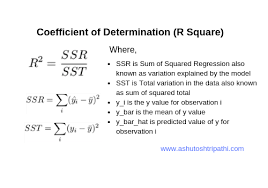
You can add a code block to calculate this R² value.
Example Code for R²:
' Calculate R² value
Dim SSresidual As Double
Dim SStotal As Double
Dim R2 As Double
' Calculate residual sum of squares (SSresidual) and total sum of squares (SStotal)
SSresidual = 0
SStotal = 0
For i = 1 To LastRow - 1
    ' Predicted Y for current X
    PredictedY = Slope * XRange.Cells(i, 1).Value + Intercept
    ' Sum of squares of residuals (observed Y - predicted Y)²
    SSresidual = SSresidual + (YRange.Cells(i, 1).Value - PredictedY) ^ 2
    ' Total sum of squares (observed Y - mean Y)²
    SStotal = SStotal + (YRange.Cells(i, 1).Value - YMean) ^ 2
Next i
' Calculate R²
R2 = 1 - (SSresidual / SStotal)
MsgBox "The R² value is: " & Round(R2, 4)
Interpreting the Model
- Slope: This represents the change in Y for each unit change in X.
- Intercept: This represents the value of Y when X = 0.
- R²: A higher R² (close to 1) means that the model explains most of the variance in the dependent variable.
Conclusion
This guide gives a basic but powerful example of how to implement a data prediction model using linear regression in Excel VBA. It demonstrates the steps to:
- Prepare the data,
- Write VBA code for regression analysis,
- Evaluate the model’s accuracy with R².
For more complex models (like multiple regression, time series forecasting, or machine learning), you would extend this approach by incorporating more variables, different formulas, or external libraries, such as integrating Python with Excel (using Power Query or Excel Python add-ins) to handle more advanced computations.
- Prepare the Data:
Implement Advanced Data Normalization Techniques with Excel VBA
Data normalization is an essential preprocessing step in data analysis and machine learning. It ensures that the data values are on a similar scale, which improves the performance of models and avoids bias caused by features with larger ranges. There are several advanced techniques for normalizing data, such as Min-Max Scaling, Z-Score Standardization, Robust Scaling, and Log Transformation. Below, I’ll explain each method and provide the VBA code to implement them in Excel.
- Min-Max Scaling
Min-Max scaling transforms the data such that it falls within a specific range, typically between 0 and 1. The formula is:
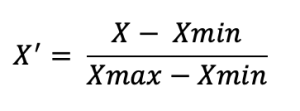
This technique is useful when we want to keep the data within a defined range, especially for algorithms like neural networks.
VBA Implementation for Min-Max Scaling:
Sub MinMaxNormalization()
    Dim ws As Worksheet
    Dim rng As Range
    Dim cell As Range
    Dim MinVal As Double
    Dim MaxVal As Double
    Dim ScaledValue As Double
    ' Set the worksheet and the range of data
    Set ws = ThisWorkbook.Sheets("Sheet1")
    Set rng = ws.Range("A2:A100") ' Modify range accordingly
    ' Find the min and max values in the range
    MinVal = Application.WorksheetFunction.Min(rng)
    MaxVal = Application.WorksheetFunction.Max(rng)
    ' Loop through each cell in the range and apply Min-Max scaling
    For Each cell In rng
        ScaledValue = (cell.Value - MinVal) / (MaxVal - MinVal)
        cell.Offset(0, 1).Value = ScaledValue ' Write the normalized value in the next column
    Next cell
End Sub
Explanation:
- The MinVal and MaxVal are computed using Excel’s Min and Max functions.
- The data is then normalized using the formula and the result is written to the next column (cell.Offset(0, 1)).
- Z-Score Standardization (Standard Scaling)
Z-Score standardization transforms the data such that the values have a mean of 0 and a standard deviation of 1. This is ideal when we want the data to be centered around 0. The formula is:
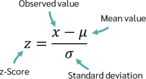
Z-Score normalization is particularly useful for algorithms like linear regression, logistic regression, and other methods sensitive to the scale of the data.
VBA Implementation for Z-Score Standardization:
Sub ZScoreStandardization()
    Dim ws As Worksheet
    Dim rng As Range
    Dim cell As Range
    Dim MeanVal As Double
    Dim StdDev As Double
    Dim ZScore As Double
    ' Set the worksheet and the range of data
    Set ws = ThisWorkbook.Sheets("Sheet1")
    Set rng = ws.Range("A2:A100") ' Modify range accordingly
    ' Calculate the mean and standard deviation
    MeanVal = Application.WorksheetFunction.Average(rng)
    StdDev = Application.WorksheetFunction.StDev(rng)
    ' Loop through each cell and apply Z-Score standardization
    For Each cell In rng
        ZScore = (cell.Value - MeanVal) / StdDev
        cell.Offset(0, 1).Value = ZScore ' Write the normalized value in the next column
    Next cell
End Sub
Explanation:
- The MeanVal is computed using the Average function, and the StdDev is calculated using StDev.
- The Z-score is computed and written to the adjacent column.
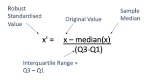
- Robust Scaling
Robust Scaling uses the median and the interquartile range (IQR) to scale the data. It is useful when the data contains outliers, as it is less sensitive to extreme values compared to Min-Max Scaling and Z-Score Standardization. The formula is:
VBA Implementation for Robust Scaling:
Sub RobustScaling()
    Dim ws As Worksheet
    Dim rng As Range
    Dim cell As Range
    Dim MedianVal As Double
    Dim Q1 As Double
    Dim Q3 As Double
    Dim IQR As Double
    Dim ScaledValue As Double
    ' Set the worksheet and the range of data
    Set ws = ThisWorkbook.Sheets("Sheet1")
    Set rng = ws.Range("A2:A100") ' Modify range accordingly
    ' Calculate the median, 25th percentile (Q1), and 75th percentile (Q3)
    MedianVal = Application.WorksheetFunction.Median(rng)
    Q1 = Application.WorksheetFunction.Percentile(rng, 0.25)
    Q3 = Application.WorksheetFunction.Percentile(rng, 0.75)
    IQR = Q3 - Q1
    ' Loop through each cell and apply Robust scaling
    For Each cell In rng
        If IQR <> 0 Then
            ScaledValue = (cell.Value - MedianVal) / IQR
            cell.Offset(0, 1).Value = ScaledValue ' Write the normalized value in the next column
        Else
            cell.Offset(0, 1).Value = 0 ' In case IQR is zero, leave the value as 0
        End If
    Next cell
End Sub
Explanation:
- The Median, Q1 (25th percentile), and Q3 (75th percentile) are computed.
- The IQR is calculated as the difference between Q3 and Q1, and the scaling is done accordingly.
- Log Transformation
Log transformation is a nonlinear transformation that is useful for reducing the skewness of the data. It works well for data that has a long-tailed distribution. The formula is:

This transformation is commonly used for datasets with exponential growth, such as financial data.
VBA Implementation for Log Transformation:
Sub LogTransformation()
    Dim ws As Worksheet
    Dim rng As Range
    Dim cell As Range
    Dim LogValue As Double
    ' Set the worksheet and the range of data
    Set ws = ThisWorkbook.Sheets("Sheet1")
    Set rng = ws.Range("A2:A100") ' Modify range accordingly
    ' Loop through each cell and apply Log transformation
    For Each cell In rng
        If cell.Value > 0 Then
            LogValue = Log(cell.Value + 1)
            cell.Offset(0, 1).Value = LogValue ' Write the normalized value in the next column
        Else
            cell.Offset(0, 1).Value = 0 ' Handle non-positive values
        End If
    Next cell
End Sub
Explanation:
- The Log function is used to apply the logarithmic transformation. We add 1 to the value to avoid the logarithm of zero or negative values.
Conclusion:
These advanced data normalization techniques—Min-Max Scaling, Z-Score Standardization, Robust Scaling, and Log Transformation—help in transforming data to a suitable range for various machine learning models and data analysis tasks.
In the provided VBA code for each technique:
- The data is processed in the specified range (A2:A100 in the example).
- Normalized values are written to the adjacent column.
Make sure you adjust the range according to your dataset. These techniques are designed to handle different data distributions and can be chosen based on the characteristics of your dataset.