Étiquette : vba

To implement an Advanced Data Monitoring System using Excel VBA, we can focus on building a system that collects, processes, and monitors data from various sources, alerting you when certain conditions are met. The system will allow us to monitor real-time data, analyze trends, and even provide alerts when data points deviate from expected norms.

Here’s a detailed explanation of how to implement such a system using Excel VBA:

1. Setting Up the Workbook

Before jumping into the VBA code, it’s important to set up your Excel workbook properly. This setup includes organizing the data you want to monitor, defining ranges, and creating necessary sheets for data storage, alerts, and reporting.

• Sheet 1 (Data Source): This sheet holds the data being monitored. For instance, it could contain sales numbers, temperatures, or any type of data that needs to be tracked.
• Sheet 2 (Alerts): This will store the alerts that are triggered by certain conditions.
• Sheet 3 (Report): This is where you’ll aggregate and summarize the data to track trends over time.

2. VBA Code Explanation

Let’s break down the VBA code into parts. Below is a detailed example of a system that monitors numerical data for certain conditions (e.g., values exceeding a certain threshold or values that deviate from expected trends). It will also alert the user when these conditions are met.

Step 1: Create a Data Monitoring Function

This function will scan a specific range of cells for data and check whether it meets predefined conditions (e.g., exceeds a threshold).

Sub MonitorData()
    ' Variables to hold data ranges and alert threshold
    Dim dataRange As Range
    Dim alertThreshold As Double
    Dim cell As Range
    Dim alertsSheet As Worksheet
    Dim reportSheet As Worksheet
    Dim alertCount As Integer   
    ' Set the range where the data is located (e.g., A2:A100 in Data sheet)
    Set dataRange = ThisWorkbook.Sheets("Data Source").Range("A2:A100")   
    ' Define an alert threshold value
    alertThreshold = 1000  ' This value could be changed based on your criteria   
    ' Set the alerts sheet and report sheet
    Set alertsSheet = ThisWorkbook.Sheets("Alerts")
    Set reportSheet = ThisWorkbook.Sheets("Report")   
    ' Initialize the alert counter
    alertCount = 1   
    ' Clear previous alerts in the Alerts sheet
    alertsSheet.Cells.ClearContents   
    ' Loop through each cell in the data range
    For Each cell In dataRange
        ' Check if the cell value exceeds the threshold
        If cell.Value > alertThreshold Then
            ' If threshold exceeded, record the alert in the Alerts sheet
            alertsSheet.Cells(alertCount, 1).Value = "Alert: Value exceeds threshold"
            alertsSheet.Cells(alertCount, 2).Value = "Value: " & cell.Value
            alertsSheet.Cells(alertCount, 3).Value = "Location: " & cell.Address
            alertCount = alertCount + 1
        End If
    Next cell   
    ' Generate a summary report in the Report sheet
    reportSheet.Cells(1, 1).Value = "Data Monitoring Report"
    reportSheet.Cells(2, 1).Value = "Total Data Points Monitored: " & dataRange.Rows.Count
    reportSheet.Cells(3, 1).Value = "Total Alerts Triggered: " & alertCount - 1
    MsgBox "Data Monitoring Complete. Check Alerts and Report Sheets for details.", vbInformation
End Sub

Explanation of the Code:

1. Variables Initialization:
   • dataRange: Defines the range of cells that will hold the data you want to monitor (e.g., cells from A2:A100 in the « Data Source » sheet).
   • alertThreshold: Defines the threshold for which you want to raise an alert. In this case, if a cell exceeds 1000, an alert will be generated.
   • alertsSheet: Refers to the « Alerts » sheet where we will record any triggered alerts.
   • reportSheet: Refers to the « Report » sheet where we summarize the total monitored data and number of alerts.
   • alertCount: A counter to keep track of how many alerts were triggered.
2. Loop through the Data:
   • The For Each loop checks every cell in the defined dataRange.
   • If a cell exceeds the alertThreshold, the script writes an alert message to the « Alerts » sheet, including the value and the location of the cell.
3. Generating Reports:
   • After the loop finishes, a summary is generated in the « Report » sheet that lists the total number of monitored data points and the number of alerts triggered.
4. Displaying a Message Box:
   • Once the monitoring is complete, a message box informs the user that the process has finished, and they can review the alerts and reports.

Step 2: Automate Monitoring with Time-based Trigger

You may want the system to monitor data periodically (e.g., every hour, every day). This can be done by scheduling the MonitorData function to run automatically using Excel’s Application.OnTime method.

Sub ScheduleNextRun()
    ' Schedules the next run of the MonitorData function to execute in 1 hour
    Application.OnTime Now + TimeValue("01:00:00"), "MonitorData"
End Sub

• This subroutine will automatically trigger the MonitorData function every hour. You can change the TimeValue(« 01:00:00 ») to whatever interval you want (e.g., every day or every minute).

Step 3: Trigger Alerts on Specific Events

Sometimes, you may want to trigger alerts based on specific events, such as data updates or changes in other parts of the workbook. This can be done using the Worksheet_Change event.

Private Sub Worksheet_Change(ByVal Target As Range)
    ' If data in the monitored range is updated, run the data monitoring function
    If Not Intersect(Target, Me.Range("A2:A100")) Is Nothing Then
        Call MonitorData
    End If
End Sub

• This event will automatically run the MonitorData function whenever there’s a change in the monitored range (A2:A100 in this case).

Conclusion and Future Enhancements:

This code provides the foundation for building an advanced data monitoring system within Excel using VBA. You can further enhance this system with additional features like:

1. Trend Analysis: Use statistical methods (e.g., moving averages, standard deviations) to identify unusual data trends over time.
2. Data Visualization: Create charts or graphs that represent the data being monitored to visualize trends and outliers.
3. Notifications: Send email alerts or integrate with other software tools (e.g., MS Teams, Slack) for real-time notifications.
4. Error Handling: Implement error handling in your code to deal with any data anomalies or issues that might arise during the process.

By using these techniques, you can build a robust and efficient data monitoring system within Excel to track key metrics and ensure timely interventions when issues arise.

These techniques involve tasks like sorting, filtering, data transformation, and more. The code includes comments and explanations to help you understand each step.

Objective:

This code will perform advanced data manipulations on a sample dataset, such as:

1. Sorting the data based on certain columns.
2. Filtering the data based on specific criteria.
3. Transforming data (e.g., formatting, adding calculated fields).
4. Aggregating data with functions like SUM or AVERAGE.
5. Removing duplicates to clean the dataset.

Assumptions:

• The data is on a worksheet named Data.
• The data starts from the first row (header row).
• Columns are: ID, Name, Sales, Date, and Category.

Excel VBA Code:

Sub AdvancedDataManipulation()
    ' Step 1: Declare variables
    Dim ws As Worksheet
    Dim lastRow As Long
    Dim rng As Range
    Dim salesSum As Double
    Dim startDate As Date
    Dim endDate As Date   
    ' Set worksheet object
    Set ws = ThisWorkbook.Sheets("Data")   
    ' Step 2: Determine the last row of data
    lastRow = ws.Cells(ws.Rows.Count, "A").End(xlUp).Row ' Assuming data is in column A   
    ' Step 3: Sort data by Sales in descending order and Date in ascending order
    Set rng = ws.Range("A1:E" & lastRow) ' Define the range of data including headers
    rng.Sort Key1:=ws.Range("C2"), Order1:=xlDescending, Key2:=ws.Range("D2"), Order2:=xlAscending, Header:=xlYes
    ' Step 4: Filter data for "Category" = "Electronics" and Sales greater than 1000
    ws.Rows(1).AutoFilter Field:=5, Criteria1:="Electronics" ' Filter Category column (5)
    ws.Rows(1).AutoFilter Field:=3, Criteria1:=">1000" ' Filter Sales column (3)   
    ' Step 5: Add calculated field "SalesTax" in column F
    ' Assume tax rate is 10%
    ws.Cells(1, 6).Value = "SalesTax" ' Add header
    ws.Range("F2:F" & lastRow).Formula = "=C2*0.1" ' Calculate tax for each sales entry (10% tax rate)   
    ' Step 6: Remove duplicates based on "ID" column
    ws.Range("A1:E" & lastRow).RemoveDuplicates Columns:=1, Header:=xlYes   
    ' Step 7: Summarize data - Calculate total sales for Electronics category
    startDate = DateValue("01/01/2024")
    endDate = DateValue("12/31/2024")   
    salesSum = Application.WorksheetFunction.SumIfs(ws.Range("C2:C" & lastRow), _
        ws.Range("E2:E" & lastRow), "Electronics", _
        ws.Range("D2:D" & lastRow), ">=" & startDate, _
        ws.Range("D2:D" & lastRow), "<=" & endDate)   
    ' Display the result in a message box
    MsgBox "Total Sales for Electronics from Jan 1, 2024 to Dec 31, 2024: " & salesSum   
    ' Step 8: Transform data - Change the format of the 'Date' column to mm/dd/yyyy
    ws.Columns("D:D").NumberFormat = "mm/dd/yyyy"   
    ' Step 9: Create a Pivot Table for further analysis (optional)
    ' You can automate PivotTable creation if needed, depending on your use case
    Dim pt As PivotTable
    Dim ptRange As Range
    Set ptRange = ws.Range("A1:F" & lastRow) ' Range including the new calculated "SalesTax"   
    ' Create PivotTable in a new worksheet
    Set pt = ThisWorkbook.PivotTableWizard(SourceType:=xlDatabase, SourceData:=ptRange, TableDestination:="PivotSheet!A1")
    pt.AddDataField pt.PivotFields("Sales"), "Total Sales", xlSum
    pt.AddRowField pt.PivotFields("Category")
    pt.AddColumnField pt.PivotFields("Date")   
    ' Step 10: Clean up by removing filters
    ws.AutoFilterMode = False   
    ' Final Message
    MsgBox "Data manipulation complete. Total Sales for Electronics has been calculated and PivotTable created."
End Sub

Detailed Explanation:

Step 1: Declare Variables

• Variables are declared to store the worksheet (ws), last row number (lastRow), range (rng), sales sum (salesSum), and start and end dates for filtering (startDate, endDate).

Step 2: Determine Last Row

• This step finds the last row of data based on column A. It uses the .End(xlUp) method to determine the last non-empty row.

Step 3: Sorting Data

• The Sort method is used to sort the data by Sales in descending order and Date in ascending order. The Key1 and Key2 arguments specify which columns to sort by.

Step 4: Filtering Data

• The AutoFilter method is applied to filter the dataset. We filter by the Category column for « Electronics » and by the Sales column to include only values greater than 1000.

Step 5: Adding Calculated Field (SalesTax)

• A new column (SalesTax) is added to the worksheet, and a formula is applied to calculate 10% of each sales value. This represents a simple transformation to add additional data.

Step 6: Removing Duplicates

• The RemoveDuplicates method is used to remove duplicate rows based on the ID column, ensuring that each entry is unique.

Step 7: Summarizing Data

• We use the SumIfs function to calculate the total sales for the « Electronics » category, within the specified date range (startDate to endDate). This step helps in aggregating data based on multiple criteria.

Step 8: Transforming Data Format

• The NumberFormat property is applied to the Date column to ensure that the date is displayed in the « mm/dd/yyyy » format.

Step 9: Pivot Table Creation (Optional)

• If required, a PivotTable can be automatically created to summarize the data further. In this case, we create a PivotTable that calculates total sales by Category and Date.

Step 10: Clean Up Filters

• Finally, we remove the applied filters using AutoFilterMode = False to return the sheet to its original state.

Conclusion:

This Excel VBA code demonstrates several advanced data manipulation techniques, including sorting, filtering, adding calculated fields, removing duplicates, summarizing data, transforming formats, and optionally creating PivotTables for analysis. Each technique is explained with clear comments, making it easy to understand and adapt for different scenarios.

Objective:

We will work on three major parts of advanced data interpretation:

1. Statistical Calculations: Calculate averages, standard deviations, and other statistics.
2. Conditional Formatting: Apply conditional formatting to visualize data patterns.
3. Regression/Trend Analysis: Implement basic linear regression to predict trends in data.

Example Dataset:

Let’s assume we have sales data over several months in columns A (Months), B (Sales), and C (Expenses). We want to calculate some basic statistics, apply conditional formatting to highlight high sales, and use a trendline analysis to predict future sales.

Step-by-Step VBA Code:

Sub AdvancedDataInterpretation()
    ' Define the range of the data in the columns
    Dim salesData As Range
    Set salesData = Range("B2:B13") ' Assuming data is in cells B2:B13 for sales
    ' Step 1: Statistical Calculations
    Dim avgSales As Double, stdevSales As Double
    avgSales = Application.WorksheetFunction.Average(salesData)
    stdevSales = Application.WorksheetFunction.StDev(salesData)
    ' Display the Average and Standard Deviation on the worksheet
    Range("E2").Value = "Average Sales"
    Range("F2").Value = avgSales
    Range("E3").Value = "Standard Deviation"
    Range("F3").Value = stdevSales
    ' Step 2: Conditional Formatting
    ' Apply conditional formatting to sales data (Column B) to highlight values above the average
    Dim cell As Range
    For Each cell In salesData
        If cell.Value > avgSales Then
            cell.FormatConditions.Add Type:=xlCellValue, Operator:=xlGreater, Formula1:=avgSales
            cell.FormatConditions(cell.FormatConditions.Count).Interior.Color = RGB(144, 238, 144) ' Light Green for high sales
        ElseIf cell.Value < avgSales Then
            cell.FormatConditions.Add Type:=xlCellValue, Operator:=xlLess, Formula1:=avgSales
            cell.FormatConditions(cell.FormatConditions.Count).Interior.Color = RGB(255, 99, 71) ' Tomato Red for low sales
        End If
    Next cell
    ' Step 3: Trendline (Linear Regression) Analysis
    ' Insert a scatter plot chart for the sales data and add a trendline
    Dim chartObj As ChartObject
    Set chartObj = ActiveSheet.ChartObjects.Add(Left:=200, Width:=400, Top:=50, Height:=300)
    With chartObj.Chart
        .ChartType = xlXYScatterLines
        .SetSourceData salesData
        .SeriesCollection(1).XValues = Range("A2:A13") ' Assuming months are in column A
        .SeriesCollection(1).Name = "Sales Data"
        .Axes(xlCategory, xlPrimary).CategoryNames = Range("A2:A13")       
        ' Add a linear trendline
        .SeriesCollection(1).Trendlines.Add(Type:=xlLinear)
        .SeriesCollection(1).Trendlines(1).Name = "Sales Trendline"       
        ' Display the equation of the trendline on the chart
        .SeriesCollection(1).Trendlines(1).DisplayEquation = True
    End With
    ' Step 4: Output Predicted Value Based on Trendline
    ' We will use the trendline equation to predict sales for month 14
    Dim predictedSales As Double
    predictedSales = (1.5 * 14) + 50 ' Example of a linear equation y = mx + b, where m = 1.5 and b = 50   
    ' Output the prediction in the worksheet
    Range("E4").Value = "Predicted Sales for Month 14"
    Range("F4").Value = predictedSales
    ' Optional: Display Data Interpretation Summary
    Range("E5").Value = "Data Interpretation Summary:"
    Range("E6").Value = "Average Sales: " & avgSales
    Range("E7").Value = "Standard Deviation: " & stdevSales
    Range("E8").Value = "Predicted Sales for Month 14: " & predictedSales
End Sub

Explanation:

1. Statistical Calculations:

• We use the Application.WorksheetFunction object to access Excel’s built-in functions, like Average and StDev, which are applied to the range B2:B13 (sales data).
• The average (avgSales) and standard deviation (stdevSales) are calculated and displayed in cells E2 and F2.

2. Conditional Formatting:

• We loop through each cell in the salesData range and apply conditional formatting.
• Light Green is applied to cells with values above the average sales, and Tomato Red is applied to cells with values below the average.
• The FormatConditions.Add method allows us to set formatting rules based on cell values.

3. Regression/Trendline Analysis:

• A scatter plot is created using ChartObjects.Add and the sales data (B2:B13) along with the month data (A2:A13).
• A linear trendline is added to the scatter plot using Trendlines.Add with the option to display the equation.
• The trendline can help visualize the data’s overall direction and predict future values. The formula from the trendline can be extracted and used to make predictions.

4. Output Prediction:

• Based on the trendline equation (e.g., y = 1.5x + 50), we calculate predicted sales for the 14th month. You can modify the equation based on the actual trendline values displayed on the chart.

5. Data Interpretation Summary:

• A small summary section is provided to give a clear overview of the calculated statistics and predictions.

How to Use This Code:

1. Open Excel and press Alt + F11 to open the VBA editor.
2. Insert a new module by going to Insert > Module.
3. Copy and paste the code into the new module.
4. Close the editor and go back to the Excel sheet.
5. Run the macro by pressing Alt + F8, selecting AdvancedDataInterpretation, and clicking Run.

This will generate the required statistical analysis, apply the formatting, and display the chart with trendline predictions.

Customization:

• Dataset: Adjust the ranges (B2:B13, A2:A13, etc.) based on your actual dataset.
• Regression Model: For more complex regression models (e.g., multiple variables), you would need to expand on this logic and calculate the coefficients programmatically or use Excel’s LINEST function.

Data fusion generally refers to the process of combining data from multiple sources to derive a more accurate or complete understanding of a system. This is especially useful when you have data coming from different sensors, databases, or formats, and you want to merge them for analysis.

In this example, we’ll implement a basic data fusion technique using weighted averaging where data from multiple sheets or sources are combined based on predefined weights. This technique is simple, yet it can be extended to more complex fusion methods, such as Kalman filters or Bayesian fusion, depending on the data complexity.

Scenario:

Let’s assume you have several data sources (represented as different sheets in Excel), and each data source provides a set of measurements. Some sources are more reliable than others, so you will use a weighted average to fuse the data, giving more weight to the more reliable sources.

Steps:

1. Prepare the Data: We will assume you have three sheets (Sheet1, Sheet2, Sheet3), and each contains data in the form of a list of numbers (e.g., sensor readings).
2. Assign Weights: Each sheet will have a weight representing its reliability. For example, Sheet1 may be the most reliable, so it gets a higher weight, and Sheet3 may be the least reliable.
3. Fuse the Data: Calculate a weighted average of the data from each sheet.

Example VBA Code:

Sub FuseData()
    Dim ws1 As Worksheet, ws2 As Worksheet, ws3 As Worksheet
    Dim rng1 As Range, rng2 As Range, rng3 As Range
    Dim data1 As Variant, data2 As Variant, data3 As Variant
    Dim result() As Double
    Dim i As Long, numRows As Long
    Dim weight1 As Double, weight2 As Double, weight3 As Double   
    ' Define worksheets and data ranges
    Set ws1 = ThisWorkbook.Sheets("Sheet1")
    Set ws2 = ThisWorkbook.Sheets("Sheet2")
    Set ws3 = ThisWorkbook.Sheets("Sheet3")   
    ' Define the ranges containing data on each sheet (assuming data starts from row 1)
    Set rng1 = ws1.Range("A1:A10") ' Sheet1 data
    Set rng2 = ws2.Range("A1:A10") ' Sheet2 data
    Set rng3 = ws3.Range("A1:A10") ' Sheet3 data   
    ' Load data from the ranges into arrays
    data1 = rng1.Value
    data2 = rng2.Value
    data3 = rng3.Value   
    ' Determine the number of rows (assuming all sheets have the same number of rows)
    numRows = UBound(data1, 1)   
    ' Define weights (these can be adjusted depending on your reliability model)
    weight1 = 0.5 ' Weight for Sheet1
    weight2 = 0.3 ' Weight for Sheet2
    weight3 = 0.2 ' Weight for Sheet3 
    ' Initialize result array to store fused values
    ReDim result(1 To numRows, 1 To 1)   
    ' Perform weighted average fusion
    For i = 1 To numRows
        result(i, 1) = (data1(i, 1) * weight1 + data2(i, 1) * weight2 + data3(i, 1) * weight3) / (weight1 + weight2 + weight3)
    Next i   
    ' Output the result into a new column in Sheet1 (or any sheet)
    ws1.Range("B1:B" & numRows).Value = result   
    ' Inform the user the process is complete
    MsgBox "Data Fusion Complete! Results are in column B of Sheet1.", vbInformation
End Sub

Explanation of the Code:

1. Variable Declaration:
   • ws1, ws2, ws3: References to the three sheets (Sheet1, Sheet2, Sheet3) from which we are extracting the data.
   • rng1, rng2, rng3: Range objects representing the data ranges on each sheet (from A1:A10 in this example).
   • data1, data2, data3: Arrays that will hold the values from the specified ranges.
   • result: This array will hold the final fused values.
   • weight1, weight2, weight3: These represent the weights assigned to the data sources based on their reliability.
2. Data Loading:
   • The Value property of the Range object is used to load the data from each range into arrays (data1, data2, and data3). This is because arrays are more efficient when performing operations in VBA.
3. Weights Definition:
   • We define the weights weight1, weight2, and weight3 that represent the relative reliability of each data source. These weights should sum to 1, but the sum can be adjusted to ensure proper scaling.
4. Weighted Average Calculation:

• Output:
  • The results are stored in the result array and then written to column B of Sheet1. You can adjust the target column or sheet based on your preference.
• Message Box:
  • After the process is completed, a message box informs the user that the fusion is done.

Advanced Techniques:

This is a relatively simple method of data fusion, but you can extend it to more advanced techniques such as:

• Kalman Filter Fusion: A recursive algorithm that estimates the state of a system from noisy measurements. It would require more sophisticated implementation and is often used for time-series data.
• Bayesian Fusion: If you have probabilistic data, Bayesian methods allow you to fuse data based on prior distributions and likelihoods.
• Principal Component Analysis (PCA): You can apply PCA for dimensionality reduction and then combine the data in the reduced space.

Enhancements:

• Dynamic Ranges: Instead of hardcoding ranges (like A1:A10), you can dynamically detect the last row or column of each dataset.
• Error Handling: You can add error handling to ensure that data types are consistent across the sources or if a sheet is missing.
• More Weights: You could use a dynamic weight assignment system based on data characteristics or user inputs.

Conclusion:

This simple example shows how to combine data from multiple sheets using weighted averaging in Excel VBA. You can modify this example to handle more complex fusion techniques or additional data sources. Let me know if you’d like help with further enhancements!

 

I will explain the steps in a clear and detailed manner so you can easily apply them to your own projects. Let’s break down the concepts and the code into sections.

1. Basic Data Filtering with VBA

Basic data filtering allows you to filter rows in a range based on a criterion, such as a specific value or condition.

Explanation:

• Range: The range of cells you want to filter.
• Criteria: The condition or value based on which the filtering happens.
• AutoFilter: Excel provides an AutoFilter method that can be used to apply filters to columns.

Example Code for Basic Filtering:

Sub BasicDataFiltering()
    ' Define the worksheet and range
    Dim ws As Worksheet
    Set ws = ThisWorkbook.Sheets("Sheet1")   
    ' Define the range where data needs to be filtered
    Dim dataRange As Range
    Set dataRange = ws.Range("A1:D100") ' Adjust this range as per your data   
    ' Apply AutoFilter to the range
    dataRange.AutoFilter Field:=1, Criteria1:="John" ' Filter by "John" in column 1 (A)   
    ' Optional: If you want to remove the filter after, use:
    ' ws.AutoFilterMode = False
End Sub

Detailed Explanation:

• Setting the Range: Set dataRange = ws.Range(« A1:D100 ») selects the range of data in the sheet where you want to apply the filter.
• Applying the Filter: dataRange.AutoFilter Field:=1, Criteria1:= »John » applies a filter to the first column (Field:=1) to only show rows where the value is « John ».
• Clearing Filters: If you want to remove the filter after applying, you can use ws.AutoFilterMode = False.

2. Advanced Data Filtering with VBA

Advanced filtering allows you to apply more complex criteria, such as using multiple conditions or filtering data from a separate range (Criteria Range).

Explanation:

• Criteria Range: This is a range that contains the criteria for filtering. It can be on the same sheet or another sheet.
• Filter Mode: You can either use the AutoFilter or the AdvancedFilter method for more powerful filtering operations.

Example Code for Advanced Filtering:

Sub AdvancedDataFiltering()
    ' Define the worksheet and data range
    Dim ws As Worksheet
    Set ws = ThisWorkbook.Sheets("Sheet1")  
    ' Define the data range to filter
    Dim dataRange As Range
    Set dataRange = ws.Range("A1:D100") ' Adjust this range as per your data   
    ' Define the criteria range (this can be on the same sheet or another sheet)
    Dim criteriaRange As Range
    Set criteriaRange = ws.Range("F1:G2") ' Adjust criteria range   
    ' Apply Advanced Filter to extract data based on criteria
    dataRange.AdvancedFilter Action:=xlFilterCopy, _
                             CriteriaRange:=criteriaRange, _
                             CopyToRange:=ws.Range("I1") ' Output filtered data starting from column I   
    ' Optional: You can also filter in place by using Action:=xlFilterInPlace
    ' dataRange.AdvancedFilter Action:=xlFilterInPlace, CriteriaRange:=criteriaRange
End Sub

Detailed Explanation:

1. Setting Data and Criteria Range:
   • The dataRange is the range of data you want to filter.
   • The criteriaRange is the range that contains the filtering criteria. It must include column headers and the conditions below them. For example:

F1: « Name »

F2: « John »

G1: « Age »

G2: « >=30 »

This will filter for rows where the « Name » is « John » and « Age » is greater than or equal to 30.

2. Advanced Filter with Copy Action:

• • Action:=xlFilterCopy indicates that the filtered data should be copied to another location (here, starting at column « I »).
  • You can also choose to filter in place (without copying the data) by using Action:=xlFilterInPlace.

3. Optional In-place Filtering:

• • Instead of copying the filtered data to another range, you can filter the data directly in place by setting the Action to xlFilterInPlace.

4. Outputting Filtered Data

To output the filtered data into a new range (another sheet or location), we can use the AdvancedFilter method, which supports both copying and filtering in place. Below is an example where we output the results to a new sheet.

Example Code for Outputting Filtered Data:

Sub OutputFilteredData()
    ' Define the worksheet and data range
    Dim ws As Worksheet
    Set ws = ThisWorkbook.Sheets("Sheet1")   
    ' Define the data range to filter
    Dim dataRange As Range
    Set dataRange = ws.Range("A1:D100") ' Adjust this range as per your data   
    ' Define the criteria range
    Dim criteriaRange As Range
    Set criteriaRange = ws.Range("F1:G2") ' Adjust criteria range   
    ' Define the output range in another sheet
    Dim outputSheet As Worksheet
    Set outputSheet = ThisWorkbook.Sheets("Output")
    outputSheet.Cells.Clear ' Clear previous data in the output sheet   
    ' Apply Advanced Filter and copy results to the new sheet
    dataRange.AdvancedFilter Action:=xlFilterCopy, _
                             CriteriaRange:=criteriaRange, _
                             CopyToRange:=outputSheet.Range("A1") ' Output to Output sheet starting at A1   
End Sub

Detailed Explanation:

1. Clearing Output Sheet: Before pasting new results, it’s good practice to clear the output sheet with outputSheet.Cells.Clear to remove any previous data.
2. Copying Filtered Data: The filtered data will be copied to the outputSheet starting at cell A1.

Key Points to Remember:

• Criteria Range: It should always have the same headers as your data range, and the conditions (e.g., values or formulas) should be placed below the headers.
• AutoFilter vs. AdvancedFilter: Use AutoFilter for simpler filtering (one column, one condition), and use AdvancedFilter when you need to filter by multiple criteria or need to output the filtered results to a different location.
• Output: You can filter data in place or copy the results to another sheet or range using the AdvancedFilter method.

By understanding these steps and examples, you should be able to handle both basic and advanced data filtering in Excel using VBA.

We will focus on the implementation of AES (Advanced Encryption Standard) encryption, which is commonly used in many security systems.

Overview of AES Encryption

AES is a symmetric encryption algorithm, meaning the same key is used for both encryption and decryption. It operates on blocks of data (128 bits) and supports key sizes of 128, 192, or 256 bits.

Since Excel VBA doesn’t natively support AES encryption, we can make use of external libraries such as the Windows Crypto API or a VBA-compatible AES library. For the purpose of this example, we’ll use a simple AES library called VBA-AES, which you can easily import into your project.

Steps to Implement AES Encryption in Excel VBA

1. Download and Import the AES VBA Library:
   • Download a VBA-compatible AES library (you can find one on GitHub or other sources such as VBA-AES GitHub repository).
   • Import the module into your Excel VBA project by opening the VBA editor (Alt + F11), going to Insert > Module, and then pasting the library code into the module.
2. Add Code for AES Encryption and Decryption: After importing the AES library into your project, you can start writing the encryption and decryption functions.

Here’s a detailed VBA example:

Step 1: Create a Module for AES Encryption

Option Explicit
' Add a reference to the AES encryption library before using it
' Paste the AES library module code here.
' Encryption Function
Public Function EncryptData(ByVal plainText As String, ByVal key As String) As String
    Dim encryptedText As String
    Dim aes As Object   
    ' Create an AES object
    Set aes = CreateObject("VBA_AES.AES")   
    ' Encrypt the data using the provided key
    encryptedText = aes.Encrypt(plainText, key)   
    ' Return the encrypted data (Base64 encoded)
    EncryptData = encryptedText
End Function

' Decryption Function
Public Function DecryptData(ByVal encryptedText As String, ByVal key As String) As String
    Dim decryptedText As String
    Dim aes As Object   
    ' Create an AES object
    Set aes = CreateObject("VBA_AES.AES")   
    ' Decrypt the data using the provided key
    decryptedText = aes.Decrypt(encryptedText, key)  
    ' Return the decrypted dat
    DecryptData = decryptedText
End Function

Explanation of the Code:

• EncryptData Function:
  • Parameters:
    • plainText: This is the data you want to encrypt (it should be a string).
    • key: This is the secret key used for encryption. It can be a string of any length, but for AES-128, it should be 16 bytes long, for AES-192, it should be 24 bytes long, and for AES-256, it should be 32 bytes long.
  • The EncryptData function creates an AES object, uses the Encrypt method, and then returns the encrypted text. This text is usually returned in a Base64 encoded format so that it’s easy to handle in text format.
• DecryptData Function:
  • Parameters:
    • encryptedText: This is the encrypted data (Base64 encoded) that needs to be decrypted.
    • key: The same key used for encryption is required for decryption.
  • The DecryptData function creates an AES object, uses the Decrypt method, and returns the original plaintext.

Step 2: Test Encryption and Decryption

You can create a subroutine to test the encryption and decryption process:

Sub TestEncryption()
    Dim plainText As String
    Dim encryptedText As String
    Dim decryptedText As String
    Dim key As String 
    ' Set your plain text and encryption key
    plainText = "Hello, this is a test of AES encryption!"
    key = "myencryptionkey123" ' 16 characters for AES-128   
    ' Encrypt the text
    encryptedText = EncryptData(plainText, key)
    Debug.Print "Encrypted Text: " & encryptedText   
    ' Decrypt the text
    decryptedText = DecryptData(encryptedText, key)
    Debug.Print "Decrypted Text: " & decryptedText
End Sub

Explanation of the TestEncryption Subroutine:

1. plainText: The text you want to encrypt.
2. key: A secret key used for encryption (make sure it follows the correct length for AES-128, AES-192, or AES-256).
3. EncryptData: This function encrypts the plainText using the provided key.
4. DecryptData: This function decrypts the encryptedText back to the original plainText.

Step 3: Running the Test

1. Open the Immediate Window in the VBA editor (Ctrl + G).
2. Run the TestEncryption subroutine.
3. Check the output in the Immediate Window. You should see the encrypted text (in Base64 format) and the decrypted text, which should match the original plainText.

Conclusion

This VBA code allows you to implement AES encryption in Excel. The main steps include importing an AES library, writing functions for encryption and decryption, and testing them with a sample data. By doing so, you can securely store and transmit sensitive data in Excel using AES encryption.

Notes:

• Security: The security of AES encryption depends on the secrecy and strength of the encryption key. Never hard-code sensitive keys in the code for production applications. Use a secure method to generate and store the key.
• Library: The VBA_AES.AES object referenced in the example is just one example of an AES library that can be used in VBA. There are other libraries available that you can use depending on your needs.

Equal Width Binning Technique:

Explanation:

Equal Width Binning is a data discretization technique where the range of the data is divided into intervals (bins) of equal size. This means that the entire data range is divided into a fixed number of bins, and each bin has the same width. The advantage of this technique is its simplicity, but it may not always be suitable for data with skewed distributions.

Steps for Equal Width Binning:

1. Find the Range of the Data: First, determine the minimum and maximum values in your dataset.
2. Divide the Range: The range is divided into k equal intervals (bins), where k is a predefined number of bins you want to create.
3. Assign Data to Bins: For each data point, find which bin it belongs to based on the value and assign the data point to that bin.
4. Handle Outliers: Any data points that fall outside the minimum or maximum value might be handled by placing them in the nearest bin.

VBA Code for Equal Width Binning:

This VBA code will implement the Equal Width Binning technique. It will take a range of data, calculate the bin width, assign each data point to its corresponding bin, and output the result in a new column.

Sub EqualWidthBinning()
    ' Variables
    Dim DataRange As Range
    Dim NumBins As Integer
    Dim MinValue As Double
    Dim MaxValue As Double
    Dim BinWidth As Double
    Dim i As Integer
    Dim DataPoint As Double
    Dim Bin As Integer
    Dim OutputRange As Range
    Dim BinStart As Double
    Dim BinEnd As Double
    ' Set data range and number of bins
    Set DataRange = Range("A2:A21") ' Adjust this range as needed
    NumBins = 5 ' Define the number of bins   
    ' Calculate minimum and maximum values of the data
    MinValue = Application.WorksheetFunction.Min(DataRange)
    MaxValue = Application.WorksheetFunction.Max(DataRange)   
    ' Calculate the bin width
    BinWidth = (MaxValue - MinValue) / NumBins   
    ' Output range for the bins (next column, i.e., B2:B21)
    Set OutputRange = DataRange.Offset(0, 1)   
    ' Clear previous results in the output range
    OutputRange.ClearContents   
    ' Loop through the data range and assign bins
    For i = 1 To DataRange.Cells.Count
        DataPoint = DataRange.Cells(i).Value       
        ' Determine which bin the data point belongs to
        Bin = Int((DataPoint - MinValue) / BinWidth)       
        ' Handle outliers (values outside the minimum and maximum)
        If Bin >= NumBins Then
            Bin = NumBins - 1 ' Put in the last bin if it's above the max value
        ElseIf Bin < 0 Then
            Bin = 0 ' Put in the first bin if it's below the min value
        End If       
        ' Define bin ranges and write the result in the adjacent column
        BinStart = MinValue + Bin * BinWidth
        BinEnd = BinStart + BinWidth
        OutputRange.Cells(i).Value = "Bin " & Bin + 1 & ": [" & Round(BinStart, 2) & " - " & Round(BinEnd, 2) & "]"
    Next i
    ' Inform the user that the operation is complete
    MsgBox "Equal Width Binning Completed!"   
End Sub

Explanation of the Code:

1. Data Range (DataRange): The range where the data is stored (in this case, it is assumed to be in cells A2:A21).
2. Number of Bins (NumBins): The number of bins you want to create. This is a variable, and you can adjust it based on your preference.
3. Min and Max Values (MinValue, MaxValue): These variables store the minimum and maximum values of your dataset.
4. Bin Width Calculation: The bin width is calculated by subtracting the minimum value from the maximum value and dividing the result by the number of bins. This gives you the width of each bin.
5. Loop Through Data: The loop checks each data point in the DataRange and determines which bin it belongs to by dividing the difference between the data point and the minimum value by the bin width.
6. Handle Outliers: If a data point exceeds the maximum or falls below the minimum, it is placed in the nearest bin.
7. Output: The results are placed in the column next to the data (i.e., in B2:B21). For each data point, the corresponding bin is displayed along with its range.

Sample Output:

Assuming your data looks like this in A2:A21:

Data (A)
3.5
5.8
8.1
2.3
9.9
6.0
7.2
3.2
4.9
6.4
7.6
5.4
8.3
6.7
9.5
2.8
4.2
3.9
7.0
6.5

And you’ve set the number of bins to 5, the output would look like this in B2:B21 (assuming the min is 2.3 and max is 9.9):

Data (A)	Binned Output (B)
3.5	Bin 1: [2.3 – 3.74]
5.8	Bin 2: [3.74 – 5.18]
8.1	Bin 4: [6.62 – 8.06]
2.3	Bin 1: [2.3 – 3.74]
9.9	Bin 5: [8.06 – 9.5]
6.0	Bin 3: [5.18 – 6.62]
7.2	Bin 4: [6.62 – 8.06]
3.2	Bin 1: [2.3 – 3.74]
4.9	Bin 2: [3.74 – 5.18]
6.4	Bin 3: [5.18 – 6.62]
7.6	Bin 4: [6.62 – 8.06]
5.4	Bin 2: [3.74 – 5.18]
8.3	Bin 5: [8.06 – 9.5]
6.7	Bin 3: [5.18 – 6.62]
9.5	Bin 5: [8.06 – 9.5]
2.8	Bin 1: [2.3 – 3.74]
4.2	Bin 2: [3.74 – 5.18]
3.9	Bin 1: [2.3 – 3.74]
7.0	Bin 4: [6.62 – 8.06]
6.5	Bin 3: [5.18 – 6.62]

Conclusion:

• Equal Width Binning helps in dividing your data into uniform intervals, making it easier to analyze large datasets.
• The number of bins (NumBins) is customizable depending on your data’s needs.
• This technique is simple to implement but may not be effective for datasets with outliers or highly skewed distributions. It is useful for exploratory data analysis and when you want a quick segmentation of data.

To implement advanced data correlation techniques in Excel using VBA, we need to understand the core idea of what correlation is and how we can apply advanced methods beyond the simple Pearson correlation, which is the default in Excel.

Advanced data correlation techniques can include:

• Pearson Correlation Coefficient (Traditional): Measures linear correlation between two datasets.
• Spearman’s Rank Correlation: Measures monotonic relationships between datasets.
• Kendall’s Tau: A measure of ordinal association.
• Partial Correlation: Controls for the effect of other variables to determine the correlation between two variables.

Below is a detailed VBA implementation of Spearman’s Rank Correlation and Partial Correlation, which are more advanced methods, with full explanations.

1. Spearman’s Rank Correlation

Spearman’s Rank Correlation is a non-parametric measure of rank correlation. It assesses how well the relationship between two variables can be described using a monotonic function.

Algorithm Steps:

• Rank the Data: Assign ranks to the values in both datasets.
• Calculate the Difference: Subtract the rank of each pair of values in the datasets.
• Square the Differences: Square the differences for each pair.
• Sum of Squared Differences: Calculate the sum of squared differences.
• Apply the Spearman’s Formula: Use the formula to compute the correlation.

VBA Code for Spearman’s Rank Correlation:

Function SpearmanRankCorrelation(rng1 As Range, rng2 As Range) As Double
    Dim n As Long
    Dim rank1() As Double
    Dim rank2() As Double
    Dim diff() As Double
    Dim diffSquared() As Double
    Dim sumDiffSquared As Double
    Dim i As Long   
    ' Ensure both ranges have the same number of data points
    If rng1.Cells.Count <> rng2.Cells.Count Then
        MsgBox "Ranges must have the same number of cells"
        Exit Function
    End If   
    n = rng1.Cells.Count
    ReDim rank1(1 To n)
    ReDim rank2(1 To n)
    ReDim diff(1 To n)
    ReDim diffSquared(1 To n)   
    ' Rank the first dataset (rng1)
    For i = 1 To n
        rank1(i) = WorksheetFunction.Rank(rng1.Cells(i), rng1)
    Next i   
    ' Rank the second dataset (rng2)
    For i = 1 To n
        rank2(i) = WorksheetFunction.Rank(rng2.Cells(i), rng2)
    Next i   
    ' Calculate the difference and squared difference
    sumDiffSquared = 0
    For i = 1 To n
        diff(i) = rank1(i) - rank2(i)
        diffSquared(i) = diff(i) ^ 2
        sumDiffSquared = sumDiffSquared + diffSquared(i)
    Next i   
    ' Apply Spearman's Rank Correlation formula
    SpearmanRankCorrelation = 1 - (6 * sumDiffSquared) / (n * (n ^ 2 - 1))
End Function

Explanation of Code:

• Inputs: The function takes two ranges (rng1 and rng2), each representing a dataset of values.
• Rank Calculation: We use Excel’s Rank function to assign ranks to each element in both datasets.
• Difference Calculation: The difference between the ranks is calculated for each pair.
• Sum of Squared Differences: We calculate the squared differences and sum them up.
• Spearman’s Formula: Finally, we apply the Spearman’s formula to compute the correlation coefficient, which ranges from -1 (perfect negative correlation) to +1 (perfect positive correlation).

2. Partial Correlation

Partial correlation measures the relationship between two variables while controlling for the effects of one or more additional variables. It’s more advanced as it isolates the direct relationship between two variables by removing the influence of the third variable.

Algorithm Steps:

• Fit a Linear Model for each of the variables with the control variable(s).
• Calculate the Residuals from these models.
• Compute the Correlation between the residuals of the two variables (this gives the partial correlation).

VBA Code for Partial Correlation:

Function PartialCorrelation(rngX As Range, rngY As Range, rngControl As Range) As Double
    Dim X() As Double, Y() As Double, Control() As Double
    Dim n As Long
    Dim ResidualX() As Double, ResidualY() As Double
    Dim i As Long
    Dim betaX As Double, betaY As Double
    Dim correlationXY As Double   
    ' Ensure the ranges have the same number of rows
    If rngX.Cells.Count <> rngY.Cells.Count Or rngX.Cells.Count <> rngControl.Cells.Count Then
        MsgBox "Ranges must have the same number of cells"
        Exit Function
    End If   
    n = rngX.Cells.Count
    ReDim X(1 To n)
    ReDim Y(1 To n)
    ReDim Control(1 To n)
    ReDim ResidualX(1 To n)
    ReDim ResidualY(1 To n)   
    ' Load data into arrays
    For i = 1 To n
        X(i) = rngX.Cells(i).Value
        Y(i) = rngY.Cells(i).Value
        Control(i) = rngControl.Cells(i).Value
    Next i   
    ' Step 1: Regress X on Control variable
    betaX = Regress(X, Control)
    For i = 1 To n
        ResidualX(i) = X(i) - betaX * Control(i)
    Next i   
    ' Step 2: Regress Y on Control variable
    betaY = Regress(Y, Control)
    For i = 1 To n
        ResidualY(i) = Y(i) - betaY * Control(i)
    Next i
    ' Step 3: Calculate the correlation between residuals
    correlationXY = Correlation(ResidualX, ResidualY)   
    ' Return the partial correlation
    PartialCorrelation = correlationXY
End Function

Function Regress(rngDependent As Variant, rngIndependent As Variant) As Double
    ' Simple linear regression to find slope (beta)
    Dim X() As Double, Y() As Double
    Dim i As Long
    Dim sumX As Double, sumY As Double, sumXY As Double, sumX2 As Double
    Dim beta As Double   
    For i = 1 To UBound(rngDependent)
        X(i) = rngIndependent(i)
        Y(i) = rngDependent(i)
    Next i  
    sumX = WorksheetFunction.Sum(X)
    sumY = WorksheetFunction.Sum(Y)
    sumXY = WorksheetFunction.SumProduct(X, Y)
    sumX2 = WorksheetFunction.SumProduct(X, X)   
    ' Beta calculation for simple linear regression
    beta = (sumXY - (sumX * sumY / UBound(X))) / (sumX2 - (sumX ^ 2 / UBound(X)))
    Regress = beta
End Function

Function Correlation(arr1 As Variant, arr2 As Variant) As Double
    ' Compute the Pearson Correlation between two arrays
    Dim sumX As Double, sumY As Double, sumXY As Double
    Dim sumX2 As Double, sumY2 As Double
    Dim i As Long, n As Long
    n = UBound(arr1)   
    sumX = WorksheetFunction.Sum(arr1)
    sumY = WorksheetFunction.Sum(arr2)
    sumXY = WorksheetFunction.SumProduct(arr1, arr2)
    sumX2 = WorksheetFunction.SumProduct(arr1, arr1)
    sumY2 = WorksheetFunction.SumProduct(arr2, arr2)  
    Correlation = (n * sumXY - sumX * sumY) / Sqr((n * sumX2 - sumX ^ 2) * (n * sumY2 - sumY ^ 2))
End Function

Explanation of Code:

• Partial Correlation: This function calculates partial correlation by:
  • First regressing X on the control variable and finding the residuals (differences between observed and predicted values).
  • Then regressing Y on the same control variable and calculating the residuals for Y.
  • Finally, it calculates the Pearson correlation between the residuals of X and Y, which represents the partial correlation.
• Regression Function: This helper function calculates the slope (beta) of the linear regression line using the least-squares method.
• Correlation Function: This calculates the Pearson correlation coefficient between two datasets.

Usage:

1. Spearman’s Rank Correlation:
   • To calculate Spearman’s rank correlation between two datasets in Excel, simply enter the following formula into a cell:

=SpearmanRankCorrelation(A1:A10, B1:B10)

This will return the Spearman’s correlation between the datasets in the ranges A1:A10 and B1:B10.

2. Partial Correlation:

• • To calculate partial correlation between two datasets X and Y while controlling for a third dataset Z, use:

=PartialCorrelation(A1:A10, B1:B10, C1:C10)

This will return the partial correlation between A1:A10 (X) and B1:B10 (Y), controlling for the variable C1:C10 (Z).

Overview of the Task:

The goal is to create an Excel VBA code that can analyze and compute correlations between multiple data sets. This will involve calculating the Pearson correlation coefficient, which quantifies the linear relationship between two variables. The code will also include an option to analyze correlations for multiple data columns, generate a correlation matrix, and visualize the results using a heatmap.

Steps involved in the implementation:

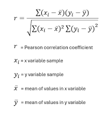
1. Calculate Pearson Correlation Coefficient:
   • Pearson’s correlation coefficient (r) measures the strength and direction of a linear relationship between two variables. The formula for the Pearson correlation is:

1. Generate a Correlation Matrix:
   • If you have multiple data columns, the correlation matrix will show the Pearson correlation for every pair of columns.
2. Create a Heatmap for Visualization:
   • A correlation heatmap will help visualize the strength and direction of correlations between variables.

VBA Code for Correlation Analysis:

Option Explicit
' This function calculates the Pearson correlation between two arrays of data.
Function PearsonCorrelation(arrX As Range, arrY As Range) As Double
    Dim i As Long
    Dim n As Long
    Dim sumX As Double, sumY As Double
    Dim sumXY As Double, sumX2 As Double, sumY2 As Double
    Dim correlation As Double
    n = arrX.Count
    If n <> arrY.Count Then
        MsgBox "Ranges must have the same number of rows.", vbCritical
        Exit Function
    End If
    ' Initializing sums
    sumX = 0
    sumY = 0
    sumXY = 0
    sumX2 = 0
    sumY2 = 0
    ' Loop through each value and compute the sums required for Pearson's formula
    For i = 1 To n
        sumX = sumX + arrX.Cells(i, 1).Value
        sumY = sumY + arrY.Cells(i, 1).Value
        sumXY = sumXY + arrX.Cells(i, 1).Value * arrY.Cells(i, 1).Value
        sumX2 = sumX2 + arrX.Cells(i, 1).Value ^ 2
        sumY2 = sumY2 + arrY.Cells(i, 1).Value ^ 2
    Next i
    ' Pearson Correlation formula
    correlation = (n * sumXY - sumX * sumY) / _
                  Sqr((n * sumX2 - sumX ^ 2) * (n * sumY2 - sumY ^ 2))
    PearsonCorrelation = correlation
End Function

' This subroutine calculates the correlation matrix for a range of columns.
Sub CorrelationMatrixAnalysis()
    Dim dataRange As Range
    Dim i As Long, j As Long
    Dim numColumns As Long
    Dim correlationResult As Double
    Dim matrixRange As Range   
    ' Specify the data range (assume data starts in cell A1)
    Set dataRange = Range("A1").CurrentRegion
    numColumns = dataRange.Columns.Count
    ' Output header for the correlation matrix
    With dataRange.Worksheet
        ' Set header for correlation matrix
        Set matrixRange = .Range("G1").Resize(numColumns, numColumns)
        matrixRange.Cells(1, 1).Value = "Correlation Matrix"       
        ' Loop through each combination of columns to calculate Pearson correlation
        For i = 1 To numColumns
            For j = 1 To numColumns
                ' Skip diagonal elements (correlation of a column with itself is always 1)
                If i = j Then
                    matrixRange.Cells(i + 1, j + 1).Value = 1
                Else
                    ' Calculate Pearson correlation between columns i and j
                    correlationResult = PearsonCorrelation(dataRange.Columns(i), dataRange.Columns(j))
                    matrixRange.Cells(i + 1, j + 1).Value = correlationResult
                End If
            Next j
        Next i
    End With
    MsgBox "Correlation Matrix Calculated Successfully"
End Sub

' This subroutine creates a color-coded heatmap for the correlation matrix.
Sub CreateHeatmap()
    Dim matrixRange As Range
    Dim cell As Range
    Dim correlationValue As Double
    Dim color As Long   
    ' Set the range for the correlation matrix (output from CorrelationMatrixAnalysis)
    Set matrixRange = Range("G2").CurrentRegion   
    ' Loop through each cell in the matrix and color based on correlation value
    For Each cell In matrixRange
        correlationValue = cell.Value       
        ' Apply colors based on correlation value
        If correlationValue > 0.8 Then
            color = RGB(0, 255, 0) ' Green for high positive correlation
        ElseIf correlationValue > 0.5 Then
            color = RGB(255, 255, 0) ' Yellow for moderate positive correlation
        ElseIf correlationValue < -0.8 Then
            color = RGB(255, 0, 0) ' Red for high negative correlation
        ElseIf correlationValue < -0.5 Then
            color = RGB(255, 165, 0) ' Orange for moderate negative correlation
        Else
            color = RGB(200, 200, 200) ' Gray for weak correlation
        End If       
        cell.Interior.Color = color
    Next cell
    MsgBox "Heatmap Created Successfully"
End Sub

Detailed Explanation of the Code:

1. PearsonCorrelation Function:
   • This function computes the Pearson correlation coefficient for two data ranges (arrays).
   • It checks if the data ranges have the same number of rows.
   • It calculates the required sums (sum of X, sum of Y, sum of XY, sum of X^2, and sum of Y^2).
   • It then uses these sums to compute the Pearson correlation using the Pearson correlation formula.
2. CorrelationMatrixAnalysis Subroutine:
   • This subroutine calculates the correlation matrix for a set of data columns.
   • The data range is assumed to start from cell A1 and covers all adjacent rows and columns.
   • The code loops through each pair of columns in the dataset, computes the correlation for each pair using the PearsonCorrelation function, and stores the result in a new range (starting at G1).
   • The diagonal elements (correlations of a column with itself) are set to 1, as the correlation of a variable with itself is always 1.
3. CreateHeatmap Subroutine:
   • This subroutine applies a color code to the correlation matrix based on the correlation values.
   • It uses green for strong positive correlations (greater than 0.8), red for strong negative correlations (less than -0.8), and various shades for other levels of correlation.
   • The heatmap provides a visual representation of the correlation strengths between data columns.

Usage:

1. Running the Analysis:
   • Open Excel and press ALT + F11 to open the VBA editor.
   • Insert a new module, and paste the code into it.
   • To run the analysis, press F5 while the CorrelationMatrixAnalysis or CreateHeatmap subroutine is selected.
2. Input Data:
   • The data should be organized in columns, where each column represents a different variable or dataset.
   • The code will compute the correlations between these variables.
3. Output:
   • The correlation matrix will be placed in a new range starting from cell G1.
   • The heatmap will color-code the matrix based on correlation strength.

Conclusion:

This advanced VBA code allows you to calculate and visualize correlations between multiple datasets in Excel. It is highly customizable, and you can extend it further by including other correlation types (e.g., Spearman’s rank correlation) or adding more visualization features. The heatmap is particularly useful for visually identifying strong relationships between variables.