Votre panier est actuellement vide !
Étiquette : vba
Find Last Column With Excel VBA
Objective:
The goal is to write a VBA code that can dynamically find the last column containing data in an Excel worksheet. This is a common task when automating data processing in Excel using VBA, especially when dealing with varying ranges where the number of columns can change.
Steps and Code:
- Understanding Excel’s Data Layout: In Excel, data can be spread out across rows and columns. While the last row can be found using methods like Cells(Rows.Count, 1).End(xlUp).Row, finding the last column requires a different approach because Excel doesn’t have a built-in function to find the last column directly.
- Strategy: We’ll use the End(xlToLeft) method, which allows us to move from a given cell (typically the farthest right cell in the row) and find the last column with data in it. This is similar to how End(xlUp) works for rows.
We’ll use the method on row 1, which is typically the header row, to determine the last column. If row 1 might be empty, we can also check the entire sheet or the used range.
- Code Explanation: Here’s the VBA code that will find the last column with data:
Sub FindLastColumn()
    Dim lastColumn As Long
    Dim ws As Worksheet
    ' Set the worksheet to the active sheet
    Set ws = ThisWorkbook.Sheets("Sheet1")
    ' Find the last column in the first row with data
    lastColumn = ws.Cells(1, ws.Columns.Count).End(xlToLeft).Column
    ' Output the result in a message box
    MsgBox "The last column with data is: " & lastColumn
End Sub
Explanation:
- Variable Declarations:
- Dim lastColumn As Long: This variable will hold the column number of the last column with data. The Long type is used because Excel supports more than 32,000 columns (up to column XFD).
- Dim ws As Worksheet: This is a reference variable to store the worksheet object.
- Setting the Worksheet:
- Set ws = ThisWorkbook.Sheets(« Sheet1 »): This line assigns the worksheet you want to work with. Replace « Sheet1 » with the name of the sheet you are working on. The ThisWorkbook keyword refers to the workbook where the macro is running.
- Finding the Last Column:
- ws.Cells(1, ws.Columns.Count).End(xlToLeft).Column: This line performs the key operation to find the last column.
- ws.Cells(1, ws.Columns.Count): This targets the last cell in row 1 (i.e., the cell in the first row and the last possible column). ws.Columns.Count returns the number of columns in the worksheet (e.g., 16384 for Excel 2010+).
- .End(xlToLeft): This moves left from the last column, stopping when it encounters the first non-empty cell. If row 1 contains data, this will move to the first column with data.
- .Column: This extracts the column number of the last cell with data.
- ws.Cells(1, ws.Columns.Count).End(xlToLeft).Column: This line performs the key operation to find the last column.
- Displaying the Result:
- MsgBox « The last column with data is: » & lastColumn: This displays a message box showing the column number of the last column with data.
Additional Notes:
- Empty Cells in the First Row: The approach above checks row 1 for the last column with data. If row 1 is empty but data is present in other rows, you can modify the code to check a different row, or use UsedRange to look at the whole sheet for the last column with data.
Example for checking the entire sheet:
lastColumn = ws.UsedRange.Columns(ws.UsedRange.Columns.Count).Column
- Used Range: The UsedRange property refers to the range of cells that have been used (i.e., that contain data). This method ensures you are looking at the range that contains data and avoids scanning the entire worksheet. However, be mindful that if cells were previously used but are now empty, UsedRange might include those columns.
- Edge Cases:
- If the first row is completely empty, this method will still work because it starts from the last possible column and works its way left.
- If there’s data in column A, for example, but not in row 1, you may need to change the row number in the code or modify it based on other criteria.
Advanced Example (Finding Last Column Based on Data in Any Row):
If you want to find the last column with data in any row, not just row 1, you can loop through the rows or check all columns in a specific range:
Sub FindLastColumnBasedOnAnyRow()
    Dim lastColumn As Long
    Dim ws As Worksheet
    Dim lastRow As Long
    Set ws = ThisWorkbook.Sheets("Sheet1")
    ' Find the last row with data
    lastRow = ws.Cells(ws.Rows.Count, 1).End(xlUp).Row
    ' Find the last column in the last row with data
    lastColumn = ws.Cells(lastRow, ws.Columns.Count).End(xlToLeft).Column
    ' Output the result
    MsgBox "The last column with data is: " & lastColumn
End Sub
Summary:
- The code provided finds the last column with data in row 1, by starting from the last column and moving left using .End(xlToLeft).
- This method is effective for scenarios where the layout of the sheet is consistent.
- For more complex data layouts, consider adjusting the code to check other rows or ranges, or use UsedRange for more flexibility.
Find and Replace Values With Excel VBA
Overview:
The goal of this code is to search for a specific value (or string) within a selected range and replace it with another value. This is very useful for cleaning up data, correcting errors, or simply updating values in a large dataset.
Key VBA Concepts:
- Range: This refers to a specific selection of cells in Excel.
- Find Method: Used to search for specific data in a range.
- Replace Method: Used to replace the found data with another value.
VBA Code for Find and Replace Values:
Sub FindAndReplaceValues()
Dim ws As Worksheet
Dim rng As Range
Dim findValue As String
Dim replaceValue As String
Dim cell As Range
' Define the worksheet you want to work with (you can specify a particular worksheet name)
Set ws = ThisWorkbook.Sheets("Sheet1")
' Define the range where you want to search (you can adjust it as needed)
Set rng = ws.Range("A1:C10")  ' Adjust the range as per your requirement
' Define the value to find and the value to replace it with
findValue = "oldValue"   ' The value you want to find
replaceValue = "newValue" ' The value you want to replace it with
' Loop through each cell in the specified range
For Each cell In rng
' Check if the current cell contains the value to find
If cell.Value = findValue Then
' Replace the value with the new value
cell.Value = replaceValue
End If
Next cell
MsgBox "Find and Replace Completed!", vbInformation
End Sub
Explanation of the Code:
- Set ws: This line sets the worksheet variable ws to the sheet you want to work with. In this case, « Sheet1 » is used, but you can replace it with any worksheet name you prefer.
- Set rng: This defines the range where the search and replacement will occur. In the example, the range is from A1 to C10. You can adjust the range depending on where you want to search for the values. If you want to search the entire sheet, you could set it as ws.UsedRange.
- findValue and replaceValue: These variables store the values you want to find and the values you want to replace them with. You can change « oldValue » and « newValue » to any values you need.
- Looping through cells: The For Each cell In rng loop goes through each cell in the specified range (rng). For every cell, it checks if the value matches the findValue.
- Check and Replace: Inside the loop, the If cell.Value = findValue checks if the current cell contains the value you are searching for. If it does, cell.Value = replaceValue replaces the found value with the new value.
- Message Box: After completing the operation, a message box appears confirming that the find and replace process is finished.
Advanced Option: Using the Find and Replace Methods
If you want to use Excel’s built-in Find and Replace methods, here’s an enhanced version of the code that uses the Range.Find method, which provides more control over the search (like searching for partial strings, match case, etc.):
Sub FindAndReplaceAdvanced()
Dim ws As Worksheet
Dim rng As Range
Dim findValue As String
Dim replaceValue As String
Dim cell As Range
Dim findCell As Range
' Define the worksheet and range
Set ws = ThisWorkbook.Sheets("Sheet1")
Set rng = ws.Range("A1:C10") ' Adjust your range accordingly
' Define the find and replace values
findValue = "oldValue"
replaceValue = "newValue"
' Use the Find method to search for the value
Set findCell = rng.Find(What:=findValue, LookIn:=xlValues, LookAt:=xlWhole, _
SearchOrder:=xlByRows, SearchDirection:=xlNext, MatchCase:=False)
' Check if the value was found
If Not findCell Is Nothing Then
' Start looping through the range from the first found cell
firstAddress = findCell.Address
Do
' Replace the found value with the new value
findCell.Value = replaceValue
' Continue to search for the next instance
Set findCell = rng.FindNext(findCell)
' Loop until all instances are replaced
Loop While Not findCell Is Nothing And findCell.Address <> firstAddress
Else
MsgBox "Value not found!"
End If
MsgBox "Find and Replace Completed!", vbInformation
End Sub
Key Changes in the Advanced Version:
- Find Method: The Find method searches for the first occurrence of the value within the specified range. It also allows you to set various search options, like case sensitivity (MatchCase) or partial matching.
- FindNext Method: This is used to continue searching for the next instance of the value after the first one is found. It ensures that every instance of the value is replaced.
- Looping Logic: The Do…Loop structure ensures that the search continues until all instances of the value have been found and replaced. The loop stops when it finds the first cell again (using the firstAddress variable).
- Error Handling: If the Find method does not find the value at all, it returns Nothing, and the code shows a message saying « Value not found! »
Key Points:
- LookIn: Determines whether to search for the value in formulas (xlFormulas), values (xlValues), or comments (xlComments).
- LookAt: Determines whether to match the entire cell content (xlWhole) or a part of it (xlPart).
- SearchDirection: Controls whether the search goes from top to bottom (xlNext) or bottom to top (xlPrevious).
- MatchCase: If True, the search is case-sensitive.
Conclusion:
This code provides a simple and flexible solution for finding and replacing values in a specified range of cells. The basic version loops through each cell manually, while the advanced version uses Excel’s built-in Find and FindNext methods for a more efficient approach, especially for large datasets.
Implement Advanced Machine Learning Models with Excel VBA
Implementing advanced machine learning models in Excel VBA is quite a challenge because VBA is not inherently designed to handle complex machine learning tasks. However, it can be used to create the structure for importing data, running simple models, and even interfacing with external libraries (such as Python or R) that specialize in machine learning.
Here’s a detailed guide on how you can use Excel VBA to implement machine learning models. We’ll focus on implementing a simple linear regression model using VBA, as an example. Then, I’ll explain how you can enhance this approach by interfacing VBA with Python or R for more advanced models.
Step 1: Prepare Data in Excel
- Organize your data: Before you implement any machine learning model, make sure your data is structured properly in Excel. For example, you might have data in the following format:
Feature1 Feature2 Target 1 2 3 2 3 5 3 4 7 … … … - Normalize/Scale Data (Optional): Depending on the complexity of your model, it might be beneficial to scale or normalize your data. For example, if you plan to implement a model like logistic regression or SVM, feature scaling might be necessary.
Step 2: Simple Linear Regression in VBA
We’ll start by implementing a simple linear regression algorithm (a type of supervised learning) using Excel VBA. This will help you get started with the basics of machine learning.
Linear Regression Formula
The linear regression model is based on the equation:
y=β0+β1×1+β2×2+⋯+βnxny
Where:
- y is the target variable
- x1,x2,…,xn are the feature variables
- β0,β1,…,βn\ are the regression coefficients (weights) that the model will learn.
To solve this, you need to calculate the values of the regression coefficients using the Ordinary Least Squares (OLS) method.
VBA Code for Linear Regression
Here’s a VBA implementation for simple linear regression with multiple features.
- Press Alt + F11 to open the VBA editor in Excel.
- Click Insert > Module to create a new module.
- Copy and paste the following code:
Sub LinearRegression()
    Dim X As Range
    Dim Y As Range
    Dim XTransposed As Range
    Dim XTX As Range
    Dim XTX_inv As Range
    Dim XTY As Range
    Dim coefficients As Range
    Dim beta As Variant
    Dim i As Integer
    Dim j As Integer
    ' Define the ranges for your data
    Set X = Range("A2:B5") ' Features (multiple columns of features)
    Set Y = Range("C2:C5") ' Target variable
    ' Step 1: Prepare the data matrix (add a column of 1s for the intercept)
    Set XTransposed = Application.WorksheetFunction.Transpose(X)
    XTransposed.Cells(1, 1).Value = 1 ' Adding the intercept (bias term)
    ' Step 2: Calculate (X'X) (Transpose of X multiplied by X)
    Set XTX = Application.WorksheetFunction.MMult(XTransposed, X)
    ' Step 3: Inverse of (X'X)
    Set XTX_inv = Application.WorksheetFunction.MInverse(XTX)
    ' Step 4: Calculate (X'Y) (Transpose of X multiplied by Y)
    Set XTY = Application.WorksheetFunction.MMult(XTransposed, Y)
    ' Step 5: Calculate the regression coefficients (Beta = (X'X)^(-1) * X'Y)
    Set coefficients = Application.WorksheetFunction.MMult(XTX_inv, XTY)
    ' Output the coefficients to the worksheet
    For i = 1 To coefficients.Rows.Count
        Cells(i, 5).Value = coefficients.Cells(i, 1).Value ' Display the coefficients in column E
    Next i
End Sub
Explanation of the Code:
- Data Preparation:
- X represents the feature matrix (the independent variables).
- Y represents the target variable (the dependent variable).
- We add a column of 1s to X to account for the intercept term (β0).
- Matrix Operations:
- XTX calculates the dot product of the transposed feature matrix (X’) and X. This is part of the OLS formula.
- XTX_inv calculates the inverse of XTX.
- XTY calculates the dot product of the transposed feature matrix (X’) and the target values Y.
- Calculate Coefficients:
- The coefficients (β0, β1, etc.) are found by multiplying the inverse of XTX with XTY.
- Display Results:
- The regression coefficients are printed in column E of the worksheet.
Step 3: Improve with Python or R Integration
While Excel VBA can handle basic regression models like the one above, it’s not the ideal environment for more complex models (like decision trees, SVMs, deep learning, etc.). For that, we can call Python or R scripts from Excel VBA.
Example: Running a Python Script from VBA
- Install Python: Ensure you have Python installed along with the necessary libraries, such as scikit-learn, pandas, and numpy.
- Create the Python Script (e.g., linear_regression.py):
import pandas as pd
from sklearn.linear_model import LinearRegression
# Read data from a CSV file (or directly from Excel)
data = pd.read_csv('data.csv')
# Separate features and target
X = data[['Feature1', 'Feature2']]
y = data['Target']
# Fit the model
model = LinearRegression()
model.fit(X, y)
# Output the coefficients
coefficients = model.coef_
intercept = model.intercept_
print("Intercept:", intercept)
print("Coefficients:", coefficients)
VBA to Call the Python Script:
Sub RunPythonScript()
    Dim objShell As Object
    Dim pythonScript As String
    Dim pythonExe As String
    ' Path to the Python executable
    pythonExe = "C:\Path\To\Python\python.exe"
    ' Path to the Python script
    pythonScript = "C:\Path\To\Script\linear_regression.py"
    ' Run the Python script
    Set objShell = CreateObject("WScript.Shell")
    objShell.Run pythonExe & " " & pythonScript, 1, True
End Sub
Step 4: Advanced Machine Learning Models
For more complex models, like decision trees, random forests, neural networks, or deep learning, Python (via scikit-learn, tensorflow, etc.) or R (via caret, randomForest, etc.) is the way to go. You can preprocess the data in Excel, export it as a CSV, and then use VBA to run the Python or R scripts.
Conclusion
This approach allows you to get started with machine learning in Excel using VBA, with linear regression as an example. Although VBA isn’t suited for complex machine learning tasks, it can serve as a useful interface to preprocess data, call external scripts, and handle simple tasks. For more advanced models, leveraging Python or R in conjunction with VBA will give you greater flexibility and power.
Implement Advanced Inventory Management Algorithms with Excel VBA
I will walk you through both concepts step by step, including how to implement them in Excel VBA.
- ABC Analysis
ABC Analysis is a method for classifying inventory into three categories (A, B, and C) based on their importance, typically using the annual consumption value.
Steps to implement ABC Analysis:
- Category A: These are the most important items, usually accounting for 70-80% of the value, but only a small percentage (10-20%) of the items.
- Category B: These items represent a moderate value, accounting for about 15-25% of the value, and 20-30% of the items.
- Category C: These are the least important, but usually make up a large percentage of the inventory in terms of volume (50-60% of items), yet only account for 5-10% of the value.
Steps to implement in VBA:
- Calculate the Annual Consumption Value for each item by multiplying the unit cost by the annual demand (usage).
- Sort items by Annual Consumption Value in descending order.
- Compute cumulative consumption percentage and classify items into A, B, or C based on their contribution to total value.
Excel VBA Code for ABC Analysis:
Sub ABCAnalysis()
    Dim ws As Worksheet
    Set ws = ThisWorkbook.Sheets("Inventory") ' Change to your sheet name
    Dim lastRow As Long
    lastRow = ws.Cells(ws.Rows.Count, "A").End(xlUp).Row ' Assuming data starts from row 2
    ' Columns (Assumed): A=Item, B=Unit Cost, C=Annual Demand, D=Annual Consumption Value, E=ABC Category
    Dim totalConsumptionValue As Double
    totalConsumptionValue = Application.WorksheetFunction.Sum(ws.Range("D2:D" & lastRow)) ' Sum of Consumption Values
    Dim cumulativeConsumptionValue As Double
    cumulativeConsumptionValue = 0
    ' Step 1: Calculate Annual Consumption Value (Unit Cost * Annual Demand)
    Dim i As Long
    For i = 2 To lastRow
        ws.Cells(i, 4).Value = ws.Cells(i, 2).Value * ws.Cells(i, 3).Value ' Annual Consumption Value (Unit Cost * Annual Demand)
    Next i
    ' Step 2: Sort the inventory by Annual Consumption Value (Column D) in descending order
    ws.Range("A1:E" & lastRow).Sort Key1:=ws.Range("D2:D" & lastRow), Order1:=xlDescending, Header:=xlYes
    ' Step 3: Calculate cumulative percentage of the total consumption value
    For i = 2 To lastRow
        cumulativeConsumptionValue = cumulativeConsumptionValue + ws.Cells(i, 4).Value
        ws.Cells(i, 5).Value = cumulativeConsumptionValue / totalConsumptionValue * 100 ' Cumulative percentage
        ' Step 4: Classify into A, B, or C based on cumulative percentage
        If ws.Cells(i, 5).Value <= 80 Then
            ws.Cells(i, 5).Value = "A"
        ElseIf ws.Cells(i, 5).Value <= 95 Then
            ws.Cells(i, 5).Value = "B"
        Else
            ws.Cells(i, 5).Value = "C"
        End If
    Next i
    MsgBox "ABC Analysis Complete!"
End Sub
Explanation of ABC Analysis Code:
- Item Classification:
- Annual Consumption Value is calculated in column D by multiplying the unit cost (column B) by the annual demand (column C).
- The data is sorted by the annual consumption value (column D), from highest to lowest.
- The cumulative consumption percentage is calculated, which is the sum of the annual consumption value divided by the total consumption value.
- The ABC classification is based on cumulative percentage:
- A: Top 70-80% of the value.
- B: Next 15-25% of the value.
- C: The remaining 5-10% of the value.
- Economic Order Quantity (EOQ)
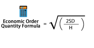
Steps to implement EOQ in VBA:
- Define the parameters: Demand (D), Ordering cost (S), and Holding cost (H).
- Calculate EOQ using the formula.
- You can also calculate the total inventory cost, which is the sum of the ordering cost and holding cost.
Excel VBA Code for EOQ Calculation:
Sub EOQCalculation()
    Dim ws As Worksheet
    Set ws = ThisWorkbook.Sheets("Inventory") ' Change to your sheet name
    Dim lastRow As Long
    lastRow = ws.Cells(ws.Rows.Count, "A").End(xlUp).Row ' Assuming data starts from row 2
    ' Columns (Assumed): A=Item, B=Annual Demand (D), C=Ordering Cost (S), D=Holding Cost (H), E=EOQ, F=Total Cost
    Dim EOQ As Double
    Dim orderingCost As Double, holdingCost As Double, demand As Double
    Dim i As Long
    For i = 2 To lastRow
        ' Step 1: Get Demand, Ordering Cost, and Holding Cost
        demand = ws.Cells(i, 2).Value
        orderingCost = ws.Cells(i, 3).Value
        holdingCost = ws.Cells(i, 4).Value
        ' Step 2: Calculate EOQ using the EOQ formula
        EOQ = Sqr((2 * demand * orderingCost) / holdingCost)
        ' Step 3: Calculate Total Cost (Ordering Cost + Holding Cost)
        ws.Cells(i, 5).Value = EOQ ' Store EOQ in column E
        ws.Cells(i, 6).Value = (demand / EOQ) * orderingCost + (EOQ / 2) * holdingCost ' Total cost in column F
    Next i
    MsgBox "EOQ Calculation Complete!"
End Sub
Explanation of EOQ Code:
- Inputs:
- Demand (D), Ordering Cost (S), and Holding Cost (H) are obtained from the spreadsheet for each item.
- EOQ Calculation: The EOQ formula is implemented using Sqr((2 * D * S) / H), and the result is stored in column E.
- Total Cost Calculation: The total inventory cost for each item is calculated as:
- Ordering Cost: DEOQ×S\frac{D}{EOQ} \times S
- Holding Cost: EOQ2×H\frac{EOQ}{2} \times H
Summary:
- The ABC Analysis helps in classifying inventory into three categories based on their importance, aiding in prioritizing items for inventory management.
- The EOQ model helps to calculate the optimal order quantity to minimize inventory costs, balancing between holding costs and ordering costs.
These two techniques are fundamental for effective inventory management and can be easily implemented in Excel VBA to automate the process.
Implement Advanced Inventory Control Algorithms with Excel VBA
The goal is to create a system that incorporates advanced inventory control techniques such as:
- Economic Order Quantity (EOQ) – Determines the optimal order quantity.
- Reorder Point (ROP) – When to place a new order to avoid stockouts.
- Safety Stock – Additional stock to prevent stockouts during demand fluctuations.
- Lead Time Demand – Calculating expected demand during lead time.
Step-by-Step Explanation:
- Economic Order Quantity (EOQ)
The EOQ formula helps us find the optimal order quantity that minimizes total inventory costs (order cost + holding cost). The formula is:
- Reorder Point (ROP)
The Reorder Point tells us when to place a new order. It depends on the lead time (time taken from placing an order to receiving it) and the average demand during this lead time.
ROP=Lead Time Demand=Lead Time×Average Demand per DayROP
3. Safety Stock
Safety Stock is an additional quantity of inventory kept to prevent stockouts due to variability in demand or lead time.
SS=Z×σL×LTSS
Where:
- Z= Service factor (based on the desired service level)
- σL = Standard deviation of demand during lead time
- LT = Lead time
- Lead Time Demand (LTD)
Lead Time Demand (LTD) is the expected demand during the lead time. This helps in predicting how much inventory will be consumed during the lead time before the next order arrives.
Excel VBA Code Implementation:
Below is an Excel VBA implementation for these advanced inventory control algorithms:
Sub AdvancedInventoryControl()
    ' Define variables for EOQ, ROP, Safety Stock, and Lead Time Demand calculations
    Dim demand As Double, orderCost As Double, holdingCost As Double
    Dim leadTime As Double, averageDemand As Double
    Dim zValue As Double, sigmaL As Double, LT As Double
    Dim eoq As Double, rop As Double, safetyStock As Double, ltd As Double
    Dim serviceLevel As Double
    ' Input values for the model (these can be replaced by cell references if needed)
    demand = 12000 ' Annual Demand (units per year)
    orderCost = 100 ' Ordering cost (per order)
    holdingCost = 5 ' Holding cost (per unit per year)
    leadTime = 7 ' Lead time (in days)
    averageDemand = 30 ' Average daily demand (units)
    ' Safety Stock parameters
    serviceLevel = 0.95 ' Desired service level (95% service level corresponds to Z=1.645)
    zValue = Application.WorksheetFunction.NormSInv(serviceLevel) ' Z value for service level
    ' Standard deviation of demand during lead time (use historical data or estimation)
    sigmaL = 10 ' Standard deviation of demand during lead time
    LT = leadTime ' Lead time in days
    ' Calculate EOQ (Economic Order Quantity)
    eoq = Sqr((2 * demand * orderCost) / holdingCost)
    ' Calculate Reorder Point (ROP)
    rop = leadTime * averageDemand
    ' Calculate Safety Stock
    safetyStock = zValue * sigmaL * Sqr(LT)
    ' Calculate Lead Time Demand (LTD)
    ltd = leadTime * averageDemand
    ' Output results to Excel sheet (or directly to the Immediate Window for debugging)
    Debug.Print "Economic Order Quantity (EOQ): " & eoq
    Debug.Print "Reorder Point (ROP): " & ro
    Debug.Print "Safety Stock: " & safetyStock
    Debug.Print "Lead Time Demand (LTD): " & ltd
    ' Optionally, output the results in specific cells (you can adjust the cell references)
    Range("B1").Value = "Economic Order Quantity (EOQ)"
    Range("B2").Value = eoq
    Range("B3").Value = "Reorder Point (ROP)"
    Range("B4").Value = ro
    Range("B5").Value = "Safety Stock"
    Range("B6").Value = safetyStock
    Range("B7").Value = "Lead Time Demand (LTD)"
    Range("B8").Value = ltd
End Sub
Explanation of the Code:
- Variable Declaration:
- Variables are declared for each of the parameters: demand, order cost, holding cost, etc. These can be replaced by cell references if you want to pull them directly from an Excel sheet.
- EOQ Calculation:
- The formula for EOQ is applied to calculate the optimal order quantity.
- ROP Calculation:
- The reorder point is calculated by multiplying the lead time by the average demand per day.
- Safety Stock Calculation:
- The safety stock is calculated using the Z-score for the desired service level and the standard deviation of demand during the lead time.
- LTD Calculation:
- Lead Time Demand is calculated simply by multiplying the average daily demand by the lead time (in days).
- Output:
- Results are output to the Immediate Window for debugging and also placed in the Excel worksheet cells for easy reference.
How to Use:
- Input Data:
- You can adjust the input values for demand, order cost, holding cost, lead time, and average demand. These values can also be linked to specific cells in an Excel sheet.
- Run the Code:
- Press Alt + F11 to open the VBA editor in Excel, then paste this code into a new module.
- You can run the AdvancedInventoryControl subroutine directly or link it to a button in your Excel sheet.
- View Results:
- The results will be displayed in the Immediate Window (for debugging) and in the Excel cells, where you can easily review the EOQ, ROP, Safety Stock, and Lead Time Demand values.
Additional Enhancements:
- Dynamic Inputs: You can set up user forms or links to cells where users can input values like demand, lead time, etc., and dynamically calculate the results.
- Inventory Tracking: You could integrate a system to track inventory levels and automatically alert when the reorder point is reached or if stock levels fall below the safety stock.
- Multiple Items: This algorithm can be expanded to work for multiple products by looping through different items and their respective inputs.
This script provides a foundational approach to implementing advanced inventory control algorithms in Excel VBA, and you can build on it depending on your specific needs and data complexity.
Implement Advanced Geospatial Analysis Techniques with Excel VBA
To implement advanced geospatial analysis techniques using Excel VBA, you need to understand a few important concepts and tools that allow you to handle and process geographical data. Geospatial analysis often involves working with spatial data, such as geographic coordinates (latitude and longitude), calculating distances, performing spatial queries, or using mapping techniques.
Since Excel VBA doesn’t come with native geospatial analysis tools like GIS software, you would typically need external libraries (such as the Geopy library in Python) or APIs (such as Google Maps API or Bing Maps API). However, Excel can still perform basic geospatial analysis, such as distance calculations, geographical transformations, and even basic mapping using VBA code.
Let’s walk through the process of implementing some advanced geospatial analysis techniques in Excel VBA, with detailed explanations of each step.
- Geospatial Data Preparation
Before performing geospatial analysis, the data should typically consist of geographical coordinates. Here is a simple setup:
ID Name Latitude Longitude 1 Place A 34.0522 -118.2437 2 Place B 40.7128 -74.0060 3 Place C 51.5074 -0.1278 You may also have additional attributes like elevation, region, or area.
- Calculating the Distance Between Two Geographical Points (Haversine Formula)
To calculate the distance between two geographical coordinates (latitude and longitude), you can use the Haversine Formula, which calculates the great-circle distance between two points on the Earth’s surface.
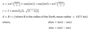
Here is the VBA code that uses the Haversine formula to calculate the distance:
Function HaversineDistance(lat1 As Double, lon1 As Double, lat2 As Double, lon2 As Double) As Double
    Dim R As Double
    Dim dLat As Double
    Dim dLon As Double
    Dim a As Double
    Dim c As Double
    ' Radius of the Earth in kilometers
    R = 6371
    ' Convert degrees to radians
    lat1 = WorksheetFunction.Radians(lat1)
    lon1 = WorksheetFunction.Radians(lon1)
    lat2 = WorksheetFunction.Radians(lat2)
    lon2 = WorksheetFunction.Radians(lon2)
    ' Differences in coordinates
    dLat = lat2 - lat1
    dLon = lon2 - lon1
    ' Haversine formula
    a = Sin(dLat / 2) ^ 2 + Cos(lat1) * Cos(lat2) * Sin(dLon / 2) ^ 2
    c = 2 * Atn(Sqr(a) / Sqr(1 - a))
    ' Calculate distance
    HaversineDistance = R * c
End Function
Explanation of the Code:
- Function Definition: The function HaversineDistance takes four parameters: the latitudes and longitudes of two locations.
- Convert to Radians: The latitudes and longitudes are converted from degrees to radians using WorksheetFunction.Radians.
- Calculate Differences: The differences in latitude and longitude are calculated.
- Haversine Formula: The formula is used to calculate the central angle between the two points.
- Distance Calculation: The final distance is calculated by multiplying the Earth’s radius by the central angle.
- Calculating the Midpoint Between Two Geographical Points
In some cases, you may want to calculate the midpoint between two geographic coordinates. The formula for calculating the midpoint is:
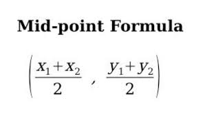
Here’s how you can implement this in VBA:
Function Midpoint(lat1 As Double, lon1 As Double, lat2 As Double, lon2 As Double) As String
    Dim midLat As Double
    Dim midLon As Double
    ' Calculate midpoint
    midLat = (lat1 + lat2) / 2
    midLon = (lon1 + lon2) / 2
    ' Return midpoint as a string
    Midpoint = "Latitude: " & midLat & ", Longitude: " & midLon
End Function
Explanation of the Code:
- The function calculates the average latitude and longitude between the two points and returns the midpoint as a string.
- Clustering Points Using K-Means Algorithm
Geospatial clustering is a common technique for identifying clusters of nearby points. One of the most widely used algorithms for clustering data is K-Means Clustering.
While implementing a full K-Means algorithm from scratch can be complex in VBA, here’s a simplified outline of how to perform clustering:
- Select the number of clusters (K).
- Randomly initialize centroids for each cluster.
- Assign each point to the nearest centroid.
- Recalculate the centroids based on the assigned points.
- Repeat steps 3-4 until convergence.
You can implement this in VBA by using arrays to store the points and centroids and iterating over the data until the algorithm converges.
- Geospatial Visualization (Using Bing Maps API)
While Excel doesn’t support interactive maps, you can visualize geospatial data by integrating Excel with the Bing Maps API (or any mapping API). The key steps are:
- Get a Bing Maps API Key from the Bing Maps portal.
- Create a URL with parameters for the map you want to show (latitude, longitude, zoom level, etc.).
- Open the Map in a Web Browser from VBA by generating a URL and using FollowHyperlink.
Example:
Sub ShowMap(lat As Double, lon As Double)
    Dim url As String
    ' Bing Maps URL format (use your actual Bing Maps API key)
    url = "https://www.bing.com/maps?cp=" & lat & "~" & lon & "&lvl=15&style=r&v=2"
    ' Open the URL in the default browser
    ThisWorkbook.FollowHyperlink url
End Sub
Explanation:
- This code generates a URL that points to a Bing Map, centered on the provided latitude and longitude.
- The map is opened in the default web browser.
Conclusion
In this example, we walked through:
- How to calculate distances between two geographical points using the Haversine formula.
- How to calculate the midpoint between two points.
- How to visualize geospatial data using the Bing Maps API.
For more advanced techniques such as spatial joins, heatmaps, or 3D geospatial visualization, you’d typically need to integrate Excel with specialized software or APIs (such as GIS software or a Python-based solution).
Implement Advanced Genetic Algorithms with Excel VBA
Implementing advanced Genetic Algorithms (GAs) in Excel VBA can be quite rewarding and challenging at the same time. Let’s break down the entire process with a detailed explanation and code.
Introduction to Genetic Algorithms (GAs)
A Genetic Algorithm (GA) is a search heuristic that is inspired by the process of natural selection. It is used to find approximate solutions to optimization and search problems. The basic idea is to mimic the process of natural evolution, where the fittest individuals are selected for reproduction to produce the offspring of the next generation.
A GA works by evolving a population of candidate solutions to a given problem. These candidates are encoded as chromosomes (a string of genes), and the evolution process involves selection, crossover (recombination), mutation, and replacement.
Steps in a Genetic Algorithm
- Initialization: Start with a randomly initialized population of solutions (chromosomes).
- Selection: Choose individuals based on their fitness to create new individuals (offspring).
- Crossover: Combine two individuals (parents) to create new offspring.
- Mutation: Randomly alter the offspring with some probability.
- Replacement: Replace the old population with the new one.
- Termination: Stop when a stopping criterion is met (e.g., number of generations, or convergence).
Problem Definition
Let’s assume you’re optimizing a simple mathematical function, such as Maximizing f(x) = x^2 where x is a binary encoded string representing a possible solution.
We’ll break down the implementation of the Genetic Algorithm in VBA for Excel.
Excel VBA Genetic Algorithm Code
Below is a detailed implementation of an advanced Genetic Algorithm using Excel VBA:
- Create a New Module in Excel VBA (Alt + F11 > Insert > Module).
- Declare the required variables and functions:
Option Explicit
' Constants
Const PopulationSize As Integer = 100        ' Population size
Const ChromosomeLength As Integer = 10       ' Number of bits in each individual
Const CrossoverRate As Single = 0.7         ' Probability of crossover
Const MutationRate As Single = 0.01         ' Probability of mutation
Const MaxGenerations As Integer = 1000      ' Max number of generations
' Data structures
Dim Population() As String
' Array to hold the population of chromosomes
Dim Fitness() As Single
' Fitness values for each chromosome
Sub GeneticAlgorithm()
    Dim Generation As Integer
    Dim BestSolution As String
    Dim BestFitness As Single
    Dim i As Integer
    Dim Parent1 As String, Parent2 As String
    Dim Child1 As String, Child2 As String
    Dim SelectedParents As Variant
    Dim NextPopulation() As String
    ' Initialize population
    Call InitializePopulation
    ' Main genetic algorithm loop
    For Generation = 1 To MaxGenerations
        ' Evaluate fitness
        Call EvaluateFitness
        ' Find best solution
        BestFitness = Application.WorksheetFunction.Max(Fitness)
        BestSolution = Population(Application.Match(BestFitness, Fitness, 0))
        ' Print the current best solution and fitness
        Debug.Print "Generation " & Generation & ": " & BestSolution & " with fitness " & BestFitness
        ' Create next generation
        ReDim NextPopulation(PopulationSize - 1)
        For i = 0 To PopulationSize - 1 Step 2
            ' Select two parents
            SelectedParents = SelectParents
            Parent1 = SelectedParents(0)
            Parent2 = SelectedParents(1)
            ' Perform crossover
            If Rnd() < CrossoverRate Then
                Call Crossover(Parent1, Parent2, Child1, Child2)
            Else
                Child1 = Parent1
                Child2 = Parent2
            End If
            ' Perform mutation
            If Rnd() < MutationRate Then Call Mutate(Child1)
            If Rnd() < MutationRate Then Call Mutate(Child2)
            ' Add children to the next population
            NextPopulation(i) = Child1
            NextPopulation(i + 1) = Child2
        Next i
        ' Update population for next generation
        Population = NextPopulation
    Next Generation
    Debug.Print "Optimization completed."
End Sub

' Initialize the population with random binary strings
Sub InitializePopulation()
    Dim i As Integer
    ReDim Population(PopulationSize - 1)
    For i = 0 To PopulationSize - 1
        Population(i) = GenerateRandomChromosome
    Next i
End Sub

' Generate a random binary chromosome of specified length
Function GenerateRandomChromosome() As String
    Dim i As Integer
    Dim Chromosome As String
    Chromosome = ""
    For i = 1 To ChromosomeLength
        If Rnd() < 0.5 Then
            Chromosome = Chromosome & "0"
        Else
            Chromosome = Chromosome & "1"
        Next i
    GenerateRandomChromosome = Chromosome
End Function

' Evaluate the fitness of each chromosome
Sub EvaluateFitness()
    Dim i As Integer
    ReDim Fitness(PopulationSize - 1)
    For i = 0 To PopulationSize - 1
        Fitness(i) = EvaluateChromosome(Population(i))
    Next i
End Sub

' Evaluate the fitness function (example: f(x) = x^2)
Function EvaluateChromosome(Chromosome As String) As Single
    Dim x As Integer
    x = BinaryToDecimal(Chromosome)
    EvaluateChromosome = x ^ 2 ' Example fitness function: f(x) = x^2
End Function

' Convert a binary string to a decimal value
Function BinaryToDecimal(Binary As String) As Integer
    Dim i As Integer
    Dim DecimalValue As Integer
    DecimalValue = 0
    For i = 1 To Len(Binary)
        DecimalValue = DecimalValue * 2 + CInt(Mid(Binary, i, 1))
    Next i
    BinaryToDecimal = DecimalValue
End Function

' Select two parents based on fitness proportionate selection
Function SelectParents() As Variant
    Dim TotalFitness As Single
    Dim SelectionPoint1 As Single, SelectionPoint2 As Single
    Dim Parent1Index As Integer, Parent2Index As Integer
    Dim Parents(1) As String
    ' Calculate total fitness
    TotalFitness = Application.WorksheetFunction.Sum(Fitness)
    ' Select two parents
    SelectionPoint1 = Rnd() * TotalFitness
    SelectionPoint2 = Rnd() * TotalFitness
    ' Find the parents by fitness
    Parent1Index = FindParentIndex(SelectionPoint1, TotalFitness)
    Parent2Index = FindParentIndex(SelectionPoint2, TotalFitness)
    Parents(0) = Population(Parent1Index)
    Parents(1) = Population(Parent2Index)
    SelectParents = Parents
End Function

' Find the index of the parent using fitness proportionate selection
Function FindParentIndex(SelectionPoint As Single, TotalFitness As Single) As Integer
    Dim i As Integer
    Dim RunningTotal As Single
    RunningTotal = 0
    For i = 0 To PopulationSize - 1
        RunningTotal = RunningTotal + Fitness(i)
        If RunningTotal >= SelectionPoint Then
            FindParentIndex = i
            Exit Function
        End If
    Next i
End Function

' Perform single-point crossover
Sub Crossover(Parent1 As String, Parent2 As String, ByRef Child1 As String, ByRef Child2 As String)
    Dim CrossoverPoint As Integer
    CrossoverPoint = Int(Rnd() * ChromosomeLength) + 1
    Child1 = Left(Parent1, CrossoverPoint) & Mid(Parent2, CrossoverPoint + 1)
    Child2 = Left(Parent2, CrossoverPoint) & Mid(Parent1, CrossoverPoint + 1)
End Sub

' Perform mutation by flipping a random bit
Sub Mutate(ByRef Chromosome As String)
    Dim MutationPoint As Integer
    MutationPoint = Int(Rnd() * ChromosomeLength) + 1
    If Mid(Chromosome, MutationPoint, 1) = "0" Then
        Mid(Chromosome, MutationPoint, 1) = "1"
    Else
        Mid(Chromosome, MutationPoint, 1) = "0"
    End If
End Sub
Explanation of the Code
- Variables and Constants:
- PopulationSize: The number of individuals in each generation.
- ChromosomeLength: The length of each individual’s chromosome (in bits).
- CrossoverRate: Probability of performing crossover.
- MutationRate: Probability of performing mutation.
- MaxGenerations: Maximum number of generations.
- Initialize Population: This creates an initial population of random binary strings (chromosomes).
- Evaluate Fitness: The fitness of each chromosome is calculated. In this case, the fitness function is f(x)=x2f(x) = x^2, where xx is the decimal representation of the binary chromosome.
- Select Parents: Two individuals (parents) are selected for reproduction based on their fitness values using fitness-proportionate selection.
- Crossover: Single-point crossover is performed to generate two offspring from the selected parents.
- Mutation: Each offspring has a chance of undergoing mutation, where one random bit in the chromosome is flipped.
- Replacement: The new generation is formed by the offspring produced through crossover and mutation, replacing the old population.
Running the Algorithm
- In the VBA editor, click Run > Run Sub/UserForm to execute the GeneticAlgorithm subroutine.
- The results (best solution and fitness per generation) will be printed to the Immediate Window (press Ctrl+G to view it).
Further Enhancements
- Custom Fitness Functions: You can modify the EvaluateChromosome function to suit more complex optimization problems.
- Elitism: You could modify the algorithm to retain the best individuals from each generation.
- Parallel Processing: For larger populations, parallelizing the evaluation of fitness could improve performance.
This is a foundational approach to implementing genetic algorithms in Excel VBA. You can further refine it by adjusting parameters, fitness functions, or introducing advanced techniques such as multi-point crossover or different selection methods.
Implement Advanced Financial Forecasting Models with Excel VBA
This example will assume that we are working on a forecast of sales for the next few years, based on historical sales data, using multiple forecasting techniques.
Explanation of Advanced Financial Forecasting
Financial forecasting involves predicting future financial outcomes based on historical data and various mathematical techniques. There are several approaches to forecasting, including:
- Moving Average: A simple forecasting model where future values are the average of the past values.
- Exponential Smoothing: A more sophisticated model that gives more weight to recent observations.
- Linear Regression: A statistical approach that uses past data to model the relationship between variables (e.g., sales and time).
- ARIMA (AutoRegressive Integrated Moving Average): A more complex time-series model.
- Monte Carlo Simulation: A method that uses random sampling to model uncertainty in forecasts.
In this VBA example, I’ll focus on the Linear Regression and Exponential Smoothing models, as they are commonly used in financial forecasting.
Data Structure
Assume that you have historical monthly sales data in columns A (Month) and B (Sales) starting from row 2.
Month Sales Jan-2020 1000 Feb-2020 1050 Mar-2020 1100 … … We will use VBA to:
- Implement a Linear Regression model to forecast future sales.
- Apply Exponential Smoothing to predict the next values.
VBA Code Implementation
Here’s a step-by-step breakdown of the code to implement these models:
Option Explicit
' This function implements Linear Regression forecasting
Function LinearRegressionForecast(rngMonths As Range, rngSales As Range, forecastPeriod As Integer) As Double
    Dim X() As Double, Y() As Double
    Dim i As Long
    Dim slope As Double, intercept As Double
    Dim forecast As Double
    ' Prepare arrays for Months and Sales data
    ReDim X(rngMonths.Rows.Count)
    ReDim Y(rngSales.Rows.Count)
    For i = 1 To rngMonths.Rows.Count
        X(i) = rngMonths.Cells(i, 1).Value ' Month values (e.g., 1 for Jan, 2 for Feb, etc.)
        Y(i) = rngSales.Cells(i, 1).Value ' Sales data
    Next i
    ' Perform Linear Regression to get Slope and Intercept (Y = mX + b)
    slope = WorksheetFunction.Slope(Y, X)
    intercept = WorksheetFunction.Intercept(Y, X)
    ' Forecasting for the next period
    forecast = (forecastPeriod * slope) + intercept
    ' Return the forecasted value
    LinearRegressionForecast = forecast
End Function

' This function implements Exponential Smoothing forecasting
Function ExponentialSmoothingForecast(rngSales As Range, smoothingFactor As Double) As Double
    Dim lastForecast As Double
    Dim i As Long
    Dim smoothedValue As Double
    ' Get the most recent sales value (use the last entry in the data)
    lastForecast = rngSales.Cells(rngSales.Rows.Count, 1).Value
    ' Apply Exponential Smoothing formula: New forecast = α * Actual value + (1 - α) * Previous forecast
    For i = rngSales.Rows.Count - 1 To 1 Step -1
        smoothedValue = smoothingFactor * rngSales.Cells(i, 1).Value + (1 - smoothingFactor) * lastForecast
        lastForecast = smoothedValue
    Next i
    ' Return the smoothed forecast
    ExponentialSmoothingForecast = lastForecast
End Function

Sub ForecastingModels()
    Dim rngMonths As Range, rngSales As Range
    Dim forecastPeriod As Integer
    Dim linearForecast As Double, expSmoothForecast As Double
    Dim smoothingFactor As Double
    ' Set the range for Months and Sales data
    Set rngMonths = Range("A2:A13") ' Modify this based on your data range
    Set rngSales = Range("B2:B13")  ' Modify this based on your data range
    ' Define forecast period (e.g., forecast for the next month)
    forecastPeriod = rngMonths.Rows.Count + 1
    ' Implement Linear Regression forecast
    linearForecast = LinearRegressionForecast(rngMonths, rngSales, forecastPeriod)
    ' Implement Exponential Smoothing forecast (alpha = 0.2)
    smoothingFactor = 0.2
    expSmoothForecast = ExponentialSmoothingForecast(rngSales, smoothingFactor)
    ' Output results
    MsgBox "Linear Regression Forecast for next month: " & linearForecast & vbCrLf & _
           "Exponential Smoothing Forecast for next month: " & expSmoothForecast
End Sub
Explanation of the Code
- Linear Regression Forecasting (LinearRegressionForecast)
- Input Parameters:
- rngMonths: A range containing the months (or time periods).
- rngSales: A range containing the historical sales data.
- forecastPeriod: The period (month) for which we are forecasting the sales.
- How it works:
- We extract the month and sales data into arrays.
- We calculate the slope and intercept using Excel’s built-in SLOPE and INTERCEPT functions.
- The forecasted sales for the specified future period are then calculated using the equation of a line: y = mx + b, where m is the slope and b is the intercept.
- Input Parameters:
- Exponential Smoothing Forecasting (ExponentialSmoothingForecast)
- Input Parameters:
- rngSales: The historical sales data.
- smoothingFactor: The smoothing constant (α), which determines the weight given to the most recent sales value.
- How it works:
- We start with the last recorded sales value as the initial forecast.
- We apply the exponential smoothing formula:
New forecast = α * Actual value + (1 – α) * Previous forecast - This is done iteratively to smooth the data.
- Input Parameters:
- The Main Subroutine (ForecastingModels)
- This subroutine calls both the LinearRegressionForecast and ExponentialSmoothingForecast functions to produce forecasts for the next period.
- The forecasted values are displayed in a message box.
How to Use the Code
- Open Excel and press Alt + F11 to open the VBA editor.
- Insert a new module by clicking Insert > Module.
- Copy and paste the above code into the module.
- Adjust the ranges (A2:A13, B2:B13) to match the location of your actual data in your Excel sheet.
- Run the ForecastingModels subroutine by pressing F5.
Conclusion
This VBA code implements a basic financial forecasting model using two techniques: Linear Regression and Exponential Smoothing. These methods are widely used in financial planning and analysis to predict future outcomes based on historical data. You can extend this model further by adding other techniques like ARIMA or Monte Carlo simulations if you need more advanced forecasting methods.
Implement Advanced Facility Location Analysis Models with Excel VBA
This example will involve solving a basic facility location problem (finding the optimal placement of facilities to minimize transportation costs) with several steps:
- Define the Problem
In a Facility Location Problem (FLP), the objective is to determine the best locations for facilities (such as warehouses, factories, etc.) to minimize costs (transportation, fixed facility costs, etc.) while considering factors like demand and capacity.
Problem Example:
- We have a set of potential facility locations (e.g., cities).
- We also have a set of customer demand points (e.g., demand locations).
- Each customer point has a demand that must be met by the nearest facility.
- We need to find the facility locations that minimize the total transportation cost.
Objective: Minimize the transportation cost
- Data Collection and Input
To implement this model, you’ll need the following inputs:
- Facility Locations (e.g., city coordinates or facility positions).
- Customer Demand Locations (e.g., customer coordinates or demand volumes).
- Distance Matrix: Calculate the distance between each facility and customer.
Input Data in Excel:
- Sheet1: Contains Facility Locations (columns A, B), where A = Facility ID, B = Facility Location (X, Y).
- Sheet2: Contains Customer Locations and Demand (columns A, B, C), where A = Customer ID, B = Customer Location (X, Y), C = Demand.
- Distance Matrix: Will be computed from the coordinates of the customers and facilities.
- Choose an Algorithm or Model
There are several approaches to solving the facility location problem:
- Greedy Algorithms
- Integer Linear Programming (ILP): Common for more complex problems.
- K-Means Clustering: Can be applied to solve facility location problems when the number of facilities is fixed.
For simplicity, let’s assume we are solving this problem using a Greedy Algorithm (the algorithm sequentially places facilities and assigns customers to minimize cost).
- Implementing in VBA
Here’s a basic implementation of a Greedy Facility Location Model in VBA:
Step-by-Step VBA Code:
Sub FacilityLocationAnalysis()
    Dim wsFacility As Worksheet, wsCustomer As Worksheet
    Dim facilityCount As Integer, customerCount As Integer
    Dim i As Integer, j As Integer
    Dim distMatrix() As Double
    Dim totalCost As Double
    Dim facilityLocation As Integer
    Dim cost As Double
    ' Set the worksheets
    Set wsFacility = ThisWorkbook.Sheets("FacilityLocations")
    Set wsCustomer = ThisWorkbook.Sheets("CustomerDemand")
    ' Get the number of facilities and customers
    facilityCount = wsFacility.Cells(Rows.Count, 1).End(xlUp).Row - 1
    customerCount = wsCustomer.Cells(Rows.Count, 1).End(xlUp).Row - 1
    ' Initialize the distance matrix (facility x customer)
    ReDim distMatrix(1 To facilityCount, 1 To customerCount)
    ' Calculate distance matrix (using Euclidean distance)
    For i = 1 To facilityCount
        For j = 1 To customerCount
            distMatrix(i, j) = CalculateDistance(wsFacility.Cells(i + 1, 2).Value, wsFacility.Cells(i + 1, 3).Value, _
                                                 wsCustomer.Cells(j + 1, 2).Value, wsCustomer.Cells(j + 1, 3).Value)
        Next j
    Next i
    ' Initialize total cost
    totalCost = 0
    ' Greedy Facility Location Selection
    For i = 1 To customerCount
        ' Find the closest facility for each customer
        facilityLocation = FindClosestFacility(distMatrix, i, facilityCount)
        ' Calculate the transportation cost for this customer-facility pai
        cost = distMatrix(facilityLocation, i) * wsCustomer.Cells(i + 1, 3).Value
        totalCost = totalCost + cost
        ' Output the result (customer and assigned facility)
        wsCustomer.Cells(i + 1, 4).Value = "Facility " & facilityLocation
        wsCustomer.Cells(i + 1, 5).Value = cost
    Next i
    ' Output the total cost
    MsgBox "Total Transportation Cost: " & totalCost
End Sub

' Function to calculate Euclidean distance
Function CalculateDistance(x1 As Double, y1 As Double, x2 As Double, y2 As Double) As Double
    CalculateDistance = Sqr((x2 - x1) ^ 2 + (y2 - y1) ^ 2)
End Function

' Function to find the closest facility to a customer
Function FindClosestFacility(distMatrix() As Double, customerIndex As Integer, facilityCount As Integer) As Integer
    Dim minDistance As Double
    Dim bestFacility As Integer
    minDistance = Application.WorksheetFunction.Max(distMatrix)
    For i = 1 To facilityCount
        If distMatrix(i, customerIndex) < minDistance Then
            minDistance = distMatrix(i, customerIndex)
            bestFacility = i
        End If
    Next i
    FindClosestFacility = bestFacility
End Function
Explanation of Code:
- Input Data:
- The facility and customer locations are assumed to be in separate worksheets: FacilityLocations and CustomerDemand.
- Distance Calculation:
- The function CalculateDistance computes the Euclidean distance between a facility and a customer. This distance is stored in a distance matrix.
- Greedy Selection:
- For each customer, the code identifies the closest facility using the FindClosestFacility function.
- The transportation cost is calculated as the distance between the facility and the customer multiplied by the demand.
- Output:
- The assigned facility for each customer is displayed in the Customer sheet, and the total transportation cost is calculated and displayed via a message box.
- Output and Visualization
After running the VBA code:
- Customer Sheet will be updated with the facility assignment and transportation cost for each customer.
- The total transportation cost will be displayed in a message box.
- To visualize the results, you can use Excel charts (e.g., scatter plot) to plot customer locations and facility locations on the same chart, with lines connecting customers to their assigned facilities.
Example Visualization:
- Scatter plot: Plot customer locations and facility locations with distinct colors.
- Lines: Draw lines connecting customers to their assigned facilities.
You can also use Excel’s Conditional Formatting to highlight the minimum cost facility assignments.
Notes:
- Complexity: This greedy approach works for small-to-medium-sized problems but may not find the global optimum. More advanced techniques like Linear Programming (via Solver) or Metaheuristics (like Genetic Algorithms) are better for larger or more complex problems.
- Scalability: For very large problems, this approach could become inefficient, and alternative methods should be considered.
- Data Input: Ensure that your data (coordinates, demand, etc.) is properly formatted in Excel to avoid errors in calculations.
Implement Advanced Decision Tree Analysis Techniques with Excel VBA
A Decision Tree is a model that is used to make decisions based on input variables. It works by splitting data into branches that represent possible outcomes. This approach is quite useful for predictive analytics, classification, and regression.
We’ll walk through the creation of a decision tree in Excel VBA, going beyond basic decision trees to include advanced techniques like pruning, cross-validation, and feature importance.
Step 1: Setting up the Excel Environment
Before diving into VBA, you should have Excel set up to use VBA. Ensure that the Developer tab is visible. If it’s not, follow these steps:
- Click on the File tab.
- Go to Options.
- In the Customize Ribbon, check the box for Developer.
Also, make sure you enable VBA macros:
- Click on Macro Security in the Developer tab.
- Set it to « Enable all macros ».
Step 2: Preparing Data
For the purpose of this example, let’s assume we are working with a classification dataset. We’ll use a simple dataset with features (independent variables) and one target variable (dependent variable).
Let’s say we have a dataset like this:
Age Income Credit Score Default 25 30k 700 No 45 50k 650 Yes 35 40k 620 No 50 60k 680 Yes 40 55k 710 No Where:
- Age, Income, and Credit Score are features.
- Default is the target variable.
Step 3: Building the Basic Decision Tree
Before diving into advanced techniques, we will start with building a basic decision tree model using Excel VBA. We will split data based on the most important feature at each node, starting with the root.
- Open Excel.
- Press Alt + F11 to open the VBA editor.
- Insert a new module (Insert > Module).
- Write the following basic VBA code to start building a Decision Tree:
Sub BuildDecisionTree()
    Dim ws As Worksheet
    Set ws = ThisWorkbook.Sheets("Data") ' Assume your data is in a sheet named "Data"
    ' Define the data range
    Dim dataRange As Range
    Set dataRange = ws.Range("A2:D6") ' Example range (A2:D6)
    ' Call the function to build a decision tree
    Call SplitNode(dataRange, 1) ' Start with root node, column 1 (Age) as the feature
End Sub

Sub SplitNode(dataRange As Range, featureIndex As Integer)
    ' Here we will use Age (feature 1) for the split
    Dim medianValue As Double
    Dim splitRange As Range
    Dim leftRange As Range, rightRange As Range
    ' Calculate the median of the feature to split
    medianValue = Application.WorksheetFunction.Median(dataRange.Columns(featureIndex))
    ' Split the data into two ranges based on the median value
    Set leftRange = dataRange.Columns(featureIndex).Resize(dataRange.Rows.Count, 1).SpecialCells(xlCellTypeVisible).Find("<=" & medianValue)
    Set rightRange = dataRange.Columns(featureIndex).Resize(dataRange.Rows.Count, 1).SpecialCells(xlCellTypeVisible).Find(">" & medianValue)
    ' Now you would perform recursion or further splitting to continue growing the tree.
    ' The function can continue splitting the data based on additional features or on different criteria.
End Sub
What happens in this code:
- The BuildDecisionTree function begins the tree-building process by calling SplitNode, which splits the data based on the Age column (feature index 1).
- In SplitNode, we find the median of the selected feature (e.g., Age) to create a binary split.
Step 4: Advanced Decision Tree Techniques
Now that we’ve seen the basics, let’s explore Advanced Decision Tree Techniques:
- Pruning
Pruning is a technique used to reduce the complexity of a decision tree by removing parts that don’t improve the model’s performance. This helps to avoid overfitting.
Here’s how we can implement pruning:
- Set a minimum sample size for leaves (e.g., 5).
- Use cross-validation to test the accuracy of the tree at each level of depth.
You could modify the code above to include a pruning condition that stops growing the tree when a node has fewer than 5 samples, for instance:
Sub SplitNodeWithPruning(dataRange As Range, featureIndex As Integer, minSamples As Integer)
    If dataRange.Rows.Count < minSamples Then Exit Sub ' Pruning condition
    ' Continue with the median split and further recursive tree building
    ' as before.
End Sub
- Cross-Validation
To avoid overfitting, cross-validation is a method of evaluating the model by splitting the data into subsets and validating the model on each.
We can implement cross-validation in VBA by splitting the dataset into, say, 5 parts, and training/testing the tree on each subset.
Sub CrossValidation(dataRange As Range, k As Integer)
    Dim foldSize As Integer
    foldSize = Int(dataRange.Rows.Count / k)
    Dim fold As Integer
    For fold = 1 To k
        ' Split the data into training and test sets
        ' Train the model on training set
        ' Test on the test set
    Next fold
End Sub
You would need to integrate this logic with your tree-building process, training the tree on each fold and measuring its accuracy.
- Feature Importance
Feature importance is a method to determine which features contribute most to the decision-making process in the tree.
A simple method to compute feature importance in decision trees is to track how much each feature reduces the impurity (like Gini impurity or entropy) at each split.
For each feature, you can calculate the total reduction in impurity across all nodes where that feature was used, and then normalize these values to determine feature importance.
Here’s a basic example of how you could track this in VBA:
Dim featureImportance As Dictionary
Set featureImportance = New Dictionary
Sub TrackFeatureImportance(featureIndex As Integer, impurityReduction As Double)
    If featureImportance.Exists(featureIndex) Then
        featureImportance(featureIndex) = featureImportance(featureIndex) + impurityReduction
    Else
        featureImportance.Add featureIndex, impurityReduction
    End If
End Sub
Step 5: Visualization of Decision Trees
While VBA is not directly used for visualizing decision trees, you can use Excel charts (e.g., scatter plots) to represent the decision boundaries visually.
For more complex visualizations like plotting decision trees as graphs, you would need external tools like Python with libraries such as matplotlib or graphviz, but this can give you a solid idea of how to build and evaluate decision trees in Excel.
Final Thoughts:
Building a decision tree in Excel VBA involves:
- Splitting data based on the best feature.
- Recursively splitting until some condition is met (e.g., maximum depth, minimum samples).
- Implementing pruning to avoid overfitting.
- Using cross-validation for more reliable performance metrics.
- Calculating feature importance to understand which features matter most.
While Excel VBA is powerful for small-scale tasks, advanced decision tree models typically use specialized software like Python (with scikit-learn) or R for better scalability, flexibility, and ease of integration with other advanced techniques.