Votre panier est actuellement vide !
Étiquette : function
How to use the YIELDDISC() function in Excel
Its calculates the annual yield of a discounted security (e.g., Treasury bills or commercial paper) that pays no periodic interest but is issued at a discount and redeemed at face value.
Syntax
YIELDDISC(Settlement; Maturity; Price; Redemption; [Basis])
Arguments
Argument Required Description Validation Rules Settlement Yes Purchase date of the security. Must be valid date < Maturity. Maturity Yes Maturity/redemption date. Must be valid date > Settlement. Price Yes Purchase price per $100 face value. Must be positive and < Redemption. Redemption Yes Redemption value per $100 face value. Typically 100. [Basis] No Day-count convention (0-4). Default=0. See Table 15-2. Error Conditions
- #VALUE!: Invalid dates.
- #NUM!: If:
- Price ≤ 0 or ≥ Redemption
- Settlement ≥ Maturity
- Basis ∉ {0,1,2,3,4}
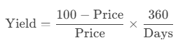
Key Formula
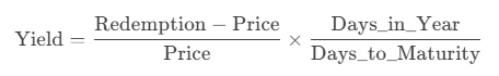
Where:
- Days_in_Year: 360 (Basis=0,2,4) or 365 (Basis=1,3).
- Days_to_Maturity: Actual calendar days between Settlement and Maturity.
Examples
- Bill of Exchange (Supplier Loan)
Scenario:
- Face Value: $5,000
- Purchase Price: $4,958.33 (5% discount)
- Settlement: 10-May-2010
- Maturity: 10-Jul-2010 (61 days)
- Basis: 4 (European 30/360)
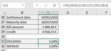
Calculation:
=YIELDDISC(« 5/10/2010 », « 7/10/2010 », 4958.33, 5000, 4)
Result: 5.04% annual yield.
Background
- Discount vs. Yield:
- Discount Rate: Anticipative interest (applied upfront).
- Yield: Equivalent interest-in-arrears return.
- Day-Count Conventions:
Basis Method Year Days 0 US (NASD) 30/360 360 1 Actual/actual 365/366 2 Actual/360 360 3 Actual/365 365 4 European 30/360 360 - Comparison with RECEIVED():
- YIELDDISC() solves for yield given price.
- RECEIVED() solves for maturity value given yield.
How to use the YIELD() function in Excel
Its calculates the annual yield of a fixed-interest security (bond) given its price, coupon rate, and maturity date. This represents the effective return an investor would earn if the bond is held to maturity.
Syntax
YIELD(Settlement; Maturity; Rate; Price; Redemption; Frequency; [Basis])
Arguments
Argument Required Description Validation Rules Settlement Yes Bond purchase date. Must be valid date < Maturity. Maturity Yes Bond maturity/redemption date. Must be valid date > Settlement. Rate Yes Annual coupon rate (decimal). ≥ 0 (e.g., 5% = 0.05). Price Yes Bond price per $100 face value. > 0 (e.g., 95.50 for $95.50). Redemption Yes Redemption value per $100 face value. Typically 100. Frequency Yes Coupon payments per year:
1 = Annual
2 = Semi-annual
4 = Quarterly.∈ {1, 2, 4}. [Basis] No Day-count convention (0-4). Default=0. See Table 15-2. Error Conditions
- #VALUE!: Invalid dates.
- #NUM!: If:
• Rate < 0 or Price ≤ 0
• Frequency ∉ {1, 2, 4}
• Basis ∉ {0, 1, 2, 3, 4}
• Settlement ≥ Maturity.
Key Formula
Solves for Yield (y) in:
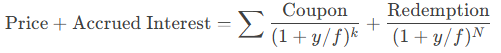
Where:
- f = Frequency
- k = Period number
- N = Total periods
Examples
- Annual Coupon Bond
Scenario:
- Settlement: 31-Aug-2010
- Maturity: 4-Jan-2013
- Coupon Rate: 4.5%
- Price: $109.01 (per $100 face value)
- Redemption: $100
- Frequency: 1 (annual)
- Basis: 1 (Actual/actual)
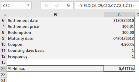
Calculation:
=YIELD(« 8/31/2010 », « 1/4/2013 », 0.045, 109.01, 100, 1, 1)
Result: 0.617% annual yield.
ISMA Yield Conversion:
=EFFECT(YIELD(…), 2)
Background
- Day-Count Conventions:
Basis Method 0 US (NASD) 30/360 1 Actual/actual 2 Actual/360 3 Actual/365 4 European 30/360 - Yield Types:
- Current Yield: Coupon/Price (simpler but less accurate).
- Yield to Maturity (YTM): Total return (what YIELD() calculates).
- Market Dynamics:
- Price < 100 → Yield > Coupon Rate (discount bond).
- Price > 100 → Yield < Coupon Rate (premium bond).
How to use the XNPV() function in Excel
Its calculates the net present value (NPV) of a series of cash flows occurring at irregular intervals, discounted at a specified annual rate. Unlike standard NPV, XNPV uses exact dates for precise time-adjusted valuation.
Syntax
XNPV(Rate; Values; Dates)
Arguments
Argument Required Description Validation Rules Rate Yes Annual discount rate (e.g., 10% = 0.10). Must be numeric. Values Yes Array of cash flows:
• Negative: Outflows (costs)
• Positive: Inflows (income).Must include ≥1 positive and ≥1 negative value. Dates Yes Exact dates corresponding to each cash flow. Dates must align with Values array; first date = start point. Error Conditions
- #VALUE!: Invalid date format.
- #NUM!: If:
• Dates/Values arrays mismatch in size
• All cash flows are positive/negative
• Dates are non-chronological.
Key Formula
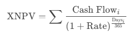
Where Days = Exact days from the first date in the series.
Example: Evaluating Discount Terms
Scenario:
A dealer offers payment terms with discounts for early payment. Compare against a 10% annual investment yield.Cash Flows:
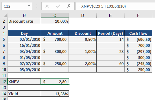
Calculation:
Effective Yield (XIRR Verification):
=XIRR({-696.5, -297, -245, 700, 300, 250}, {« 1/2/2010 », « 4/3/2010 », « 7/7/2010 », « 1/16/2010 », « 5/1/2010 », « 9/7/2010 »})
Result: 13.58% (beats 10% alternative).
Why Use XNPV?
- Precision: Accounts for exact days between cash flows (e.g., 14 days vs. « 1 month »).
- Flexibility: Evaluates irregular income/expenditures (e.g., project milestones, custom payment plans).
- Decision Tool:
- Positive NPV: Project/investment adds value.
- Negative NPV: Reconsider or adjust terms.
Comparison with NPV
Feature XNPV NPV Timing Exact dates Equal intervals Formula Daily compounding (365) Periodic compounding Use Case Leases, trade credit Annuities, loans How to use the XIRR() function in Excel
Its calculates the internal rate of return (IRR) for a series of cash flows with irregular timing, providing the annualized effective return rate.
Syntax
XIRR(Values; Dates; [Guess])
Arguments
Argument Required Description Validation Rules Values Yes Array of cash flows (positive for inflows, negative for outflows). Must include at least one positive and one negative value. Dates Yes Corresponding dates for each cash flow. Dates must be in chronological order after the first date. [Guess] No Initial estimate for IRR (default=10%). Helps convergence in complex scenarios. Error Conditions
- #VALUE!: Invalid date format.
- #NUM!: If:
- Dates not chronological
- Mismatched array sizes
- No solution found (e.g., all positive/negative cash flows)
Background
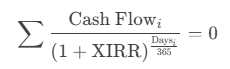
XIRR extends the classic IRR by accommodating irregular intervals, using daily compounding based on a 365-day year. It solves for the discount rate that sets the net present value (NPV) of cash flows to zero:
Examples
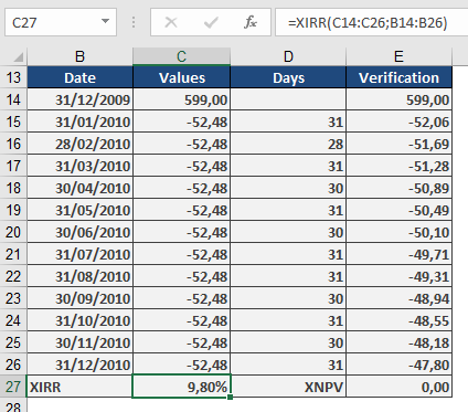
- Consumer Loan Evaluation
Scenario:
- Washing machine: $599 (initial outflow, entered as -599)
- 12 monthly payments: $52.48 (inflows, entered as +52.48)
Calculation:
=XIRR({-599, 52.48, 52.48, …, 52.48}, {« 1/1/2023 », « 2/1/2023 », …, « 12/1/2023 »})
Result: 9.8% effective annual rate.
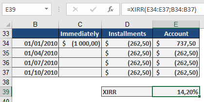
- Insurance Premium Financing
Scenario:
- Annual premium: $1,000
- Quarterly alternative: 4 payments of $262.50
Calculation:
=XIRR({737.50, -262.50, -262.50, -262.50, -262.50}, {« 1/1/2023 », « 4/1/2023 », « 7/1/2023 », « 10/1/2023 », « 1/1/2024 »})
Result: 14.2% implied annual cost.
Key Features
- Real-World Applicability:
- Evaluates loans, investments, or leases with flexible payment schedules.
- Adjusts for exact calendar days (e.g., 28-day vs. 31-day months).
- Comparison Tool:
- Compare financing options (e.g., lump-sum vs. installments).
- Annualizes returns for irregular cash flows (e.g., venture capital).
- Limitations:
- Requires at least one inflow and one outflow.
- May fail with highly irregular cash flows (adjust Guess if needed).
How to use the VDB() function in Excel
Its Calculates depreciation for an asset using the declining balance method, with an optional switch to straight-line depreciation when advantageous. This flexible approach is commonly used for tax purposes.
Syntax
VDB(Cost; Salvage; Life; Start_Period; End_Period; [Factor]; [No_Switch])
Arguments
Argument Required Description Validation Rules Cost Yes Initial asset value (purchase price + expenses). Must be positive. Salvage Yes Asset value at end of depreciation. Must be ≥ 0 and < Cost. Life Yes Useful life in periods (integer). Must be > 0. Start_Period Yes Starting period for depreciation calculation. Must be < Life. End_Period Yes Ending period for depreciation calculation. Must be ≥ Start_Period. [Factor] No Accelerated depreciation rate (default=2 for double-declining). Typically 1.5–2. [No_Switch] No FALSE (default): Switches to straight-line when optimal; TRUE: Forces declining balance. Logical (TRUE/FALSE). Error Conditions
- #VALUE!: Non-numeric inputs.
- #NUM!: If:
- Cost ≤ 0 or Salvage < 0
- Life ≤ 0 or Start_Period ≥ Life
- Factor ≤ 0
Background
The Variable Declining Balance (VDB) method combines:
- Accelerated Depreciation: Higher expenses in early years (e.g., double-declining balance).
- Automatic Switch to Straight-Line: When straight-line depreciation exceeds the declining balance amount.
Key Formula
Depreciation=Book Value×(FactorLife)Depreciation=Book Value×(LifeFactor)
- Book Value = Cost – Accumulated Depreciation.
- Switch Condition: If straight-line depreciation > declining balance, VDB switches.
Example
Asset Depreciation:
- Cost: $1,000
- Salvage: $100
- Life: 10 years
- Factor: 2 (double-declining)
- No_Switch: FALSE (auto-switch enabled)
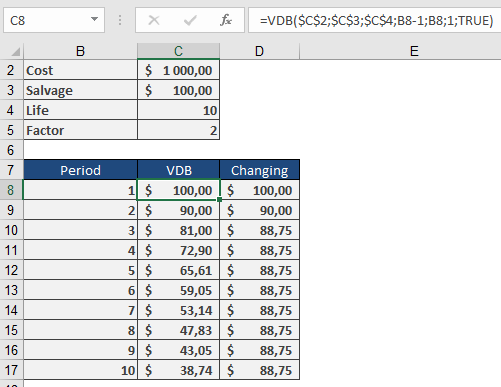
Depreciation Schedule
Year Method Depreciation Book Value 1 Double-Declining $200.00 $800.00 2 Double-Declining $160.00 $640.00 3 Double-Declining $128.00 $512.00 4 Straight-Line* $103.00 $409.00 … … … … *Switches to straight-line in Year 4 when it becomes more beneficial.
Key Features
- Tax Optimization: Maximizes early-year deductions.
- Flexibility: Adjust Factor for local tax rules (e.g., 1.5× for mid-range acceleration).
- Partial Periods: Combine with manual adjustments for mid-year purchases.
Complementary Functions
- DB(): Fixed declining balance (no switch).
- DDB(): Double-declining balance (no switch).
- SLN(): Straight-line depreciation.
How to use the TBILLYIELD() function in Excel
Its calculates the yield to maturity of a U.S. Treasury bill (T-bill) as an annualized percentage, based on the purchase price and time to maturity.
Syntax
TBILLYIELD(Settlement; Maturity; Price)
Arguments
Argument Required Description Validation Rules Settlement Yes Trade settlement date (purchase date). Must be valid date < Maturity. Maturity Yes Maturity/redemption date. Must be ≤ 1 year after Settlement. Price Yes Purchase price per $100 face value. Must be positive and < 100 (discounted). Error Conditions
- #VALUE!: Invalid date format.
- #NUM!: If:
- Settlement ≥ Maturity
- Maturity > 1 year after Settlement
- Price ≤ 0 or ≥ 100
Background
T-bills are zero-coupon securities sold at a discount. The yield represents the annualized return if held to maturity.
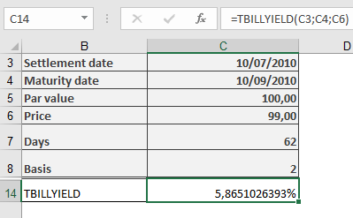
Key Formula
Where:
- Days = Actual calendar days between Settlement and Maturity.
- Uses 360-day year (consistent with U.S. banking conventions).
Example
T-Bill Investment:
Key Notes
- Comparison with Other Functions
- YIELDDISC(Basis=2) matches TBILLYIELD().
- RECEIVED() calculates maturity value, not yield.
- Practical Use
- Compare T-bill returns with other short-term investments.
- Adjusts for the 360-day banking year (no compounding).
- Limitations
- Only valid for T-bills with maturities ≤ 1 year.
- Price must be < 100 (discounted securities).
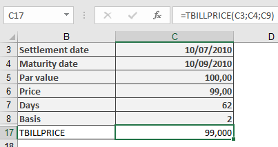
How to use the TBILLPRICE() function in Excel
Its calculates the price per $100 face value of a U.S. Treasury bill (T-bill) based on its discount rate. T-bills are short-term securities that are issued at a discount and mature at par value.
Syntax
TBILLPRICE(Settlement; Maturity; Discount)
Arguments
Argument Required Description Validation Rules Settlement Yes The trade settlement date Must be valid date < Maturity Maturity Yes The maturity/redemption date Must be ≤ 1 year after Settlement Discount Yes The annual discount rate (decimal) Must be > 0 Error Conditions
- #VALUE!: Invalid date format
- #NUM!: If:
- Settlement ≥ Maturity
- Maturity > 1 year after Settlement
- Discount ≤ 0
Calculation Method
The price is calculated using:
Price = 100 × (1 – Discount × D/360)
Where:
- D = Number of days between Settlement and Maturity
- Uses actual calendar days (Basis = 2 equivalent)
Example
Key Features
- Day Count Convention: Uses actual/360 (Basis = 2)
- Output Format: Returns price as percentage of par value
- Complementary Functions:
- TBILLYIELD(): Calculates yield from price
- PRICEDISC(): Similar but allows different day count bases
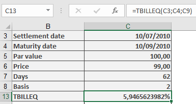
How to use the TBILLEQ() function in Excel
Its Calculates the bond-equivalent yield (annualized return) for a U.S. Treasury bill (T-bill) based on its discount rate, converting the T-bill’s discount yield (360-day basis) to an equivalent investment yield (365-day basis).
Syntax
TBILLEQ(Settlement; Maturity; Discount)
Arguments
Argument Required Description Validation Rules Settlement Yes Trade date (when T-bill is purchased). Must be a valid date < Maturity. Maturity Yes Maturity date (when T-bill is redeemed). Must be ≤ 1 year after Settlement. Discount Yes Discount rate (as a decimal, e.g., 5% = 0.05). Must be > 0. Error Conditions
- #VALUE!: Invalid dates.
- #NUM!: If:
- Settlement ≥ Maturity
- Maturity > 1 year after Settlement
- Discount ≤ 0
Background
T-bills are zero-coupon securities sold at a discount and redeemed at par. The TBILLEQ function converts the discount rate (used to price T-bills) into an equivalent annual yield (used to compare returns with other investments).
Key Formula
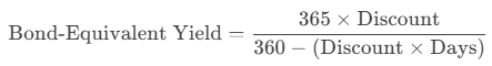
Where:
- Days = Actual days between Settlement and Maturity.
Example
Key Notes
- Comparison with Other Functions
- YIELDDISC(): Returns the yield directly (no 365-day conversion).
- RECEIVED(): Calculates maturity value, not yield.
- Practical Use
- Compare T-bill returns with bonds or savings accounts.
- Adjusts for the 360-day banking year used in T-bill pricing.
- Limitations
- Only valid for T-bills with maturities ≤ 1 year.
- Does not account for compounding.
How to use the SYD() function in Excel
Its calculates the depreciation of an asset for a specified period using the sum-of-the-years’ digits (SYD) method, an accelerated depreciation technique that applies higher depreciation expenses in earlier periods.
Syntax
SYD(Cost; Salvage; Life; Per)
Arguments
Argument Required Description Validation Rules Cost Yes Initial asset cost (purchase price + additional expenses – discounts). Must be a positive value. #VALUE! if non-numeric, invalid if negative. Salvage Yes Asset value at the end of its useful life. Must be ≥ 0. #VALUE! if non-numeric, #NUM! if negative. Life Yes Total depreciation periods (integer > 0). Must be a positive integer. Per Yes Specific period for depreciation calculation (integer > 0). Must be ≤ Life. Background
Depreciation reflects the reduction in an asset’s value over time. The SYD method applies a declining depreciation expense each period, unlike straight-line depreciation.
Key Features
- Accelerated Depreciation: Higher expenses in early years, decreasing over time.
- Formula:
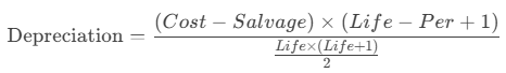
-
- Numerator: Remaining useful life at the start of the period.
- Denominator: Sum of the years’ digits (e.g., 5 years → 1+2+3+4+5 = 15).
- Tax & Accounting Use:
- Permitted in some jurisdictions for tax benefits.
- Not suitable for all assets (check local regulations).
Example
Asset Details:
- Cost: $1,000
- Salvage Value: $0
- Life: 5 years
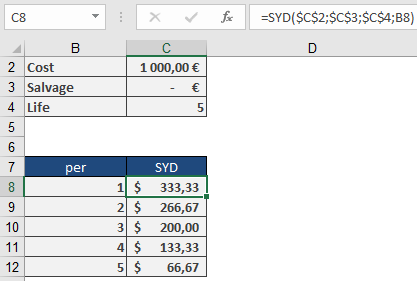
Depreciation Schedule:
Year Calculation (SYD) Depreciation Book Value 1 =SYD(1000,0,5,1) $333.33 $666.67 2 =SYD(1000,0,5,2) $266.67 $400.00 3 =SYD(1000,0,5,3) $200.00 $200.00 4 =SYD(1000,0,5,4) $133.33 $66.67 5 =SYD(1000,0,5,5) $66.67 $0.00 Key Takeaway:
- Year 1 has the highest depreciation ($333.33).
- Year 5 has the lowest ($66.67).
Implementation Notes
- Partial-Year Depreciation:
- SYD assumes full periods. Adjust manually for mid-year purchases.
- Complementary Functions:
- SLN(): Straight-line depreciation.
- DDB(): Double-declining balance (more aggressive than SYD).
- Best Practices:
- Use ROUND(SYD(…), 2) for financial reporting precision.
- Verify tax compliance before applying SYD.
How to use the SLN() function in Excel
Its calculates straight-line depreciation for an asset over a specified period, allocating equal depreciation expense in each accounting period.
Syntax
SLN(Cost; Salvage; Life)
Arguments
Argument Required Description Validation Rules Cost Yes Initial asset value (purchase price + incidental costs) Must be positive Salvage Yes Asset value at end of depreciation Must be ≥ 0 Life Yes Useful life in periods Must be integer > 0 Error Conditions
- #VALUE!: Non-numeric inputs
- #NUM!: Negative values or invalid Life
Calculation Method
Annual Depreciation = (Cost – Salvage) / Life
Key Features
- Equal Periodic Charges: Allocates depreciation evenly across all periods
- Common Applications:
- Financial reporting
- Tax calculations (where permitted)
- Budget forecasting
Example
Asset Depreciation Scenario:
- Purchase cost: $1,000
- Salvage value: $100
- Useful life: 5 years
Calculation:
=SLN(1000, 100, 5)
Result: $180 per year
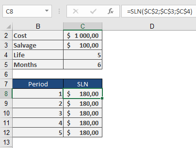
Depreciation Schedule:
Year Beginning Value Depreciation Ending Value 1 $1,000 $180 $820 2 $820 $180 $640 3 $640 $180 $460 4 $460 $180 $280 5 $280 $180 $100 Implementation Notes
- First-Year Convention:
- For partial-year depreciation, manually adjust first period
- Use SLN() for subsequent full periods
- Best Practices:
=ROUND(SLN(Cost, Salvage, Life), 2)
Ensures compliance with financial reporting standards
- Complementary Functions:
- DB(): Declining balance method
- DDB(): Double-declining balance
- SYD(): Sum-of-years’ digits
Technical Considerations
- Tax Compliance:
- Verify local regulations permit straight-line method
- Some jurisdictions require accelerated methods
- Asset Management:
- Combine with physical depreciation tracking
- Useful for capital budgeting analysis