Votre panier est actuellement vide !
Catégorie : Excel function
How to use the DMAX function in Excel
This function returns the largest numerical value from a specified column within a list or database, based on conditions that you define.
Syntax
DMAX(database; field; criteria)
Arguments
- database (required): This is the cell range that makes up your list or database.
- field (optional): This indicates which column the function should use.
- criteria (required): This is the cell range containing the field names and the filter criteria you want to apply.
Background
Use the DMIN() and DMAX() functions to find the smallest or largest value in a database based on specific criteria. DMAX() will return a value from a database, such as the highest production volume for a product over the last five years.
Example
As a wholesaler, you have many customers and sell a wide range of products. You want to analyze your customers, sales, and products. Let’s start by finding the product and customer with the highest sales based on orders within the United States. You can achieve this using the DMAX() function.
The DMAX() function will search for the largest sales value for orders originating from the United States (see Figure below). Since you only want to know the highest sales within the United States, you’ll specify « USA » as a search criterion (B5). You won’t specify a product because you want to include all products in your search.
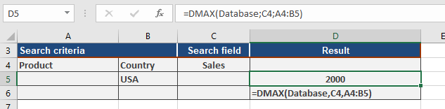
DMAX() will then return 2000, meaning the highest single order placed in the United States was for $2,000.
If you also want to know which company placed this order and what product they bought, you can perform additional calculations using the DGET() function. Figure below shows one way to do this.
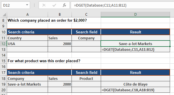
With the DMAX() function, you can quickly analyze your sales and customers.
How to use the DGET function in Excel
This function extracts a single value from a specified column within a list or database, based on conditions that you define.
Syntax
DGET(database; field; criteria)
Arguments
- database (required): This is the cell range that constitutes your list or database.
- field (optional): This indicates which column the function should use for extracting the value.
- criteria (required): This is the cell range that contains the field names and the filter criteria you wish to apply.
Background
To find a specific value within a database where a particular field matches certain criteria, use the DGET() function.
Example
Imagine you’re a wholesaler and you’ve received a complaint from a customer, « Old World Delicatessen. » They claim the tofu they ordered is moldy. To submit a complaint to the manufacturer and inquire about any known production issues, you need to find out the exact date you sold that tofu to « Old World Delicatessen. » The DGET() function can help you do this. Since « Old World Delicatessen » definitely ordered the tofu, you can be sure that DGET() will return a result.
DGET() returns 12/3/2007 when using the company name, country/region, and item number as criteria (as shown in B4:D5 in Figure below). By using the DGET() function, you can quickly retrieve values from your database, even when you specify multiple search criteria.

How to use the DCOUNTA function in Excel
This function counts the number of non-empty cells within a specified column, list, or database that match the given conditions.
Syntax
DCOUNTA(database; field; criteria)
Arguments
- database (required): This is the cell range that defines your list or database.
- field (optional): This indicates which column the function should use.
- criteria (required): This is the cell range containing the field names and the filter criteria.
Background
DCOUNTA() is different from DCOUNT() because it counts non-empty cells, whereas DCOUNT() specifically counts numerical values.
Example
Let’s say your business is relatively new, and you want to find out how many invoices were sent to companies in the United States. You also need the total number of invoices in your database to calculate the percentage of invoices sent to U.S. companies.
First, open a new worksheet and define your criteria range using the « Country/Region » field from your original data. Then, specify « USA » as your search criterion (see Figure below).
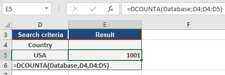
Since DCOUNTA() counts text, it will return the number of records that match « USA ». For the database argument, specify the cell range containing your database, such as A1:F7008. In this example, that cell range is dynamically named « Database ».
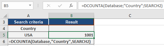
You’ll get the same result if you enter « SEARCH2 » for the criteria range (A4:A5 in this example) and input « country/region » instead of cell A4 in the field argument. Just remember to enclose the field name, « country/region », in quotation marks.
The result will still be 1001; this means your database contains 1,001 records matching the « USA » criterion, indicating that 1,001 invoices were sent to companies in the United States (see Figure below).
Now, to calculate the total number of invoices issued, you’ll do it the same way. The search range remains unchanged, but to count all records in the « country » search range, refer the search criterion to an empty cell (see Figure below).
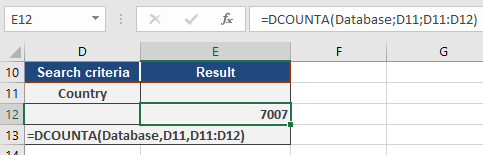
After you’ve calculated a total of 7,007 for all invoices, you can then figure out the percentage of invoices sent to companies within the United States. As shown in Figure below, you can calculate this percentage using the DCOUNTA() function.

Although this method might seem a bit tedious, it’s effective. You’ll find that 14 percent of your invoices go to companies in the United States, with the remaining invoices sent to companies outside th.e U.S
How to use the DCOUNT function in Excel
This function counts the number of records that contain numerical values in the specified field column, provided they match the defined conditions.
Syntax
DCOUNT(database; field; criteria)
Arguments
- database (required): This is the cell range that identifies your list or database.
- field (optional): This indicates which column the function will use for counting. You can enter the column label enclosed in quotation marks (e.g., « country/region », « sales », or « company »). Alternatively, you can use a number representing the column’s position within the list (e.g., 1 for the first column, 2 for the second, and so on).
- criteria (required): This is the cell range that holds your field names and the filter criteria. Any range can be used for the criteria argument, as long as it includes at least one column label and at least one cell below that label where you specify a condition for the column.
Background
The DCOUNT() function performs a simple task, but it can be a huge time-saver, especially when you’re working with databases and need to count many records. Use the DCOUNT() function to count records that contain numbers and match specific criteria within a database.
Example
Imagine you’re a wholesaler and you want to know how many deliveries have been invoiced. This means you want to count all sales that are greater than zero.
First, open a new worksheet and define your criteria range using the « Sales » field from your original data. Then, specify the search criterion as >0.
Now, use the DCOUNT() function to calculate the number of sales in your database that are greater than zero (see Figure below).

For the database argument, specify the named range « Database », which refers to A1:F7008. In this example, using a dynamic name like « Database » saves you from having to type the cell range A1:F7008 every time you refer to your database.
As you can see in Figure below, you’ll get the same result if you enter the name « SEARCH1 » for the criteria range (A11:A12 in the figure) and specify « Sales » instead of cell A11 for the field argument. Remember to enclose the field name, « Sales », in quotation marks. As shown in Figure below, the result remains 7,000.

This means your database contains 7,000 records for sales greater than zero. You can quickly count sales greater than 1,500 in the same way.
How to use the DAVERAGE function in Excel
This function calculates the arithmetic mean for values within a list or database column that meet specified conditions.
Syntax
DAVERAGE(database; field; criteria)
Arguments
- database (required): The cell range that constitutes the list or database.
- field (optional): Specifies which column the function will use.
- criteria (required): The cell range that contains the field names and the filter criteria.
Background
The arithmetic mean is the most commonly recognized mean value. Its ease of calculation makes it crucial for summarizing and analyzing data. To compute the mean, values in a range are summed, and then the sum is divided by the total number of values.
Use the DAVERAGE() function to calculate the mean for selected database records.
Example
It’s year-end, and you’re analyzing sales. Specifically, you want to determine the average sales of products in various countries. The DAVERAGE() function can help you calculate these values.
To find the average sales for « Chang » in the United States, you would specify « USA » as the country/region and « Chang » as the item name. Since you’re looking for average sales, you’d use « Sales » as the database field. DAVERAGE() would then return $1,522.85 (refer to Figure below).

You also want to calculate the overall average sales for « Chang ». To do this for « Chang » across all countries and regions, simply omit the country/region as a search criterion. This ensures all countries and regions are included in the calculation. DAVERAGE() will return $1,560.02 as the average sales order value (refer to Figure below).

By using the DAVERAGE() function, you can effectively compare the average sales for products across different countries.
How to use the TYPE function in Excel
This function returns a number indicating the data type of the specified value.
Syntax: TYPE(value)
Arguments:
- value (required): The expression to check (a number, text, a formula without an equal sign, a logical value, an error value, a reference, or a name).
Background:
- The TYPE() function is related to the IS() functions, which return logical values based on the argument’s type.
- It is often used with IF() to pre-test calculation results, and its output can support conditional formatting and data validation rules.
- To use this function effectively, refer to the mappings in Table 1.
Table 1. Data Types Mapped to Numbers
Argument Return Value Number 1 Text 2 Logical value 4 Error value 16 Array 64 Key Notes:
- Except for arrays, the results can also be obtained using ISNUMBER(), ISTEXT(), ISNONTEXT(), ISLOGICAL(), and ISERROR(). For example:
- ISNUMBER(B12) and TYPE(B12) = 1 are logically equivalent.
- Limitations:
- ISBLANK(), ISNA(), ISREF(), and ISERR() (which excludes #N/A) are incompatible with TYPE().
- TYPE() cannot detect whether a cell contains a formula—it only returns the result’s data type.
- For array formulas, TYPE() returns 64 only if the argument is a range entered with Ctrl+Shift+Enter.
Examples:
- Replicating IS() Functions:
- Replace =ISERROR(B3) with =(TYPE(B3)=16).
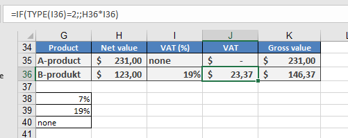
- Replace =IF(ISTEXT(I36);;H36*I36) with =IF(TYPE(I36)=2;;H36*I36).
How to use the NA function in Excel
This function returns the #N/A error value, indicating that a value does not exist.
Syntax: NA
Arguments:
- This function does not take any arguments.
Background:
- Although the NA() function does not require arguments, you must include the parentheses; otherwise, Excel will interpret it as text.
- Similar to TRUE() and FALSE(), where you can directly enter logical values (TRUE or FALSE), you can also manually enter #N/A instead of using NA() to achieve the same result.
- This function is primarily included for compatibility with other spreadsheet applications.
Usage Notes:
- You can use NA() (or #N/A) to explicitly mark empty cells, ensuring they are excluded from calculations.
- However, formulas referencing cells containing #N/A will also return the error, so use this function with caution.
Example:
- In the example for the ISBLANK() function, empty cells were checked to exclude them from calculations. If NA() were used instead, the desired result would not be obtained.
- Scenario:
- Column C references Column B, and the average is calculated in cell D2.
- If C3 contained a 0, it would not match Column B, so the empty cell in B is marked as =NA() or #N/A.
- However, the #N/A error propagates into all calculations.
Workaround:
=IF(ISNA(B7), « », B7)
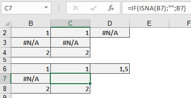
This formula returns the correct result, similar to what the ISBLANK() function would provide.
How to use the N FUNCTION in Excel
This function returns a value converted into a number.
Syntax. N(value)
Arguments
- value (required). The expression (a number, text, a formula without an equal sign, a logical value, an error value, a reference, or a name) that you want to convert into a number.
Background. Usually, you don’t need to use the N() function because Excel automatically converts values when a number is required. However, the IS() functions are an exception. For compatibility with other spreadsheet software, this function remains available.
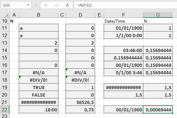
The N() function converts expressions as shown in Table 1.
Table 1. Conversion Results with the N() Function
Argument (Expression) Return Value Number The same number Date Serial number for the date Time Number for the time TRUE 1 FALSE 0 Error value The same error value Text or an empty cell 0 Example. For examples of this function’s usage, see the « Time Basics » Inside Out sidebar in this chapter.
How to use the ISTEXT function in Excel
Returns TRUE if the value is text (including numeric strings like « 123 »). Returns FALSE for numbers, errors, logical values, empty cells, or empty strings (« »).
Syntax
ISTEXT(value)
Key Behavior
Input Type ISTEXT Result Notes Regular text TRUE « Apple », « 123 » Empty cell FALSE Number FALSE 100, 3.14 Boolean FALSE TRUE/FALSE Error FALSE #N/A, #VALUE! Empty string (« ») FALSE Result of formulas like = » » Practical Applications
- Sales Tax Calculation (Text vs. Number)
Scenario: Column M contains either text (e.g., « Exempt ») or tax rates (e.g., 7%).
=IF(ISTEXT(M42); « »; L42*M42)
- Text in M42 → Returns blank (« »)
- Number in M42 → Calculates L42*M42
- Data Validation (Text-Only Fields)
Restrict cell input to text:
- Select cell → Data → Data Validation → Custom
- Formula:
=ISTEXT(A1)
- Clean Mixed Data
Identify text entries in a column:
=IF(ISTEXT(B2), « Text », « Not Text »)
Special Notes
- Numeric Strings:
- ISTEXT(« 100 ») → TRUE
- ISTEXT(100) → FALSE
- Empty vs. Zero:
- Blank cell → FALSE
- Formula returning « » → FALSE
- Counterpart:
ISTEXT(value) = NOT(ISNONTEXT(value))
Example Walkthrough
Problem: Calculate gross values where tax rates may be text (« Exempt ») or numbers (7%, 19%).
Solution:
=IF(ISTEXT(M42); ; L42*M42)
- If M42 is « Exempt » → Skips calculation (returns blank)
- If M42 is 0.07 (7%) → Multiplies by L42

Data Validation Setup:
- Create a list of valid inputs (e.g., « Exempt », 7%, 19%) in another sheet (e.g., column K).
- Apply to column M:
- Data → Data Validation → List
- Source: =$K$1:$K$3
Pro Tip
Combine with TRIM() to handle spaces:
=ISTEXT(TRIM(A1)) // Returns FALSE for cells with only spaces
How to use the ISREF function in Excel
Returns TRUE if the value is a valid cell reference (including named ranges). Returns FALSE for all other inputs (numbers, text, invalid references).
Syntax
ISREF(value)
Key Features
What Returns TRUE?
✔ Standard references (A1, Sheet2!B5)
✔ Named ranges (« Sales Data »)
✔ Structured references (Table1[Column1])What Returns FALSE?
✖ Numbers/text (123, « A1 »)
✖ Formulas (SUM(A1:A10))
✖ Invalid references (-B1, XYZ!A1 for non-existent sheets)Special Cases
⚠ Returns TRUE for references to non-existent sheets/tables (e.g., SheetX!A1), as Excel only validates syntax, not existence.
Practical Applications
- Safeguarding Named Ranges
Prevent #NAME? errors when a named range might be deleted:
=IF(ISREF(ABC), AVERAGE(ABC), « Error: Named range ‘ABC’ was deleted »)
- Dynamic Formula Validation
Check if a cell contains a valid reference before using:
=IF(ISREF(INDIRECT(B1)), « Valid reference », « Invalid input »)
- Conditional Formatting
Highlight cells containing references:
=ISREF(A1) // Applies formatting to reference-containing cells
Example Breakdown
Scenario
A workbook uses a named range ABC for calculations. To avoid #NAME? errors if ABC is deleted:
Original (Risky):
=AVERAGE(ABC) // Fails with #NAME? if ABC is deleted
Protected Version:
=IF(ISREF(ABC), AVERAGE(ABC), « removed Named ABC « )
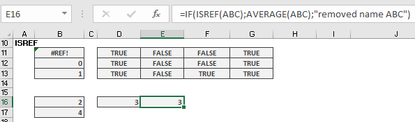
Behaviour:
- If ABC exists → Returns average
- If ABC is deleted → Shows friendly message
Limitations
- Cannot detect circular references or broken links.
- Returns TRUE for syntactically valid but non-existent references (e.g., Sheet99!A1).
For robust reference checking, combine with other functions like IFERROR() or ISERROR().