Votre panier est actuellement vide !
Catégorie : Excel function
How to use the CUBEMEMBERPROPERTY function in Excel
This function returns the property of a member from the cube. Use CUBEMEMBERPROPERTY() to validate that a member exists within the cube and to return the property for this member as a value.
Syntax
CUBEMEMBERPROPERTY(connection; member_expression; property)
Arguments
- connection (required): A string representing the name of the workbook connection to the cube. After you type the first quotation mark, existing context-sensitive data connections are displayed.
- member_expression (required): Defines the position of a member in the cube based on a Multidimensional Expression (MDX). The expression can be entered directly or referenced from a cell. Tuples can also be used in expressions.
- property (required): The name of the property for which you want to return the value.
Background
In the example in this section, the stores have the « Group » property with possible values of « North » or « South ».
While the data is being queried, the message #GETTING_DATA temporarily appears in the cell containing the function.
Error values and messages provide information about incorrect or missing entries:
- If the connection name is not a valid workbook connection, the CUBEMEMBERPROPERTY() function returns the #NAME? error.
- If the OLAP server (or the offline cube) is unavailable, an error message will appear, but the content of the affected cell will not change.
- If the member_expression syntax is incorrect, or if the member specified by member_expression does not exist in the cube, the CUBEMEMBERPROPERTY() function returns the #N/A error.
- CUBEMEMBERPROPERTY() might also return the #N/A error when the connection to the data source is interrupted and cannot be re-established.
Example
As previously mentioned, the stores in the PivotTable have the « Group » properties « North » and « South. »
The formula =CUBEMEMBERPROPERTY(« offline », »[Stores].[Store Name].[All].[NorthEast] », »group Name ») returns North.
The formula =CUBEMEMBERPROPERTY(« offline », »[Stores].[Store].&[3] », »group ») returns South.
This example uses the position number of the store in the list instead of the store name.

CUBEMEMBER()
Syntax
CUBEMEMBER(connection; member_expression; caption)
Definition
This function returns a member (cell) from a cube. Use CUBEMEMBER() to validate the existence of a member and to pass that member to other functions via a cell reference.
Arguments
- connection (required): The text string name of the workbook connection to the cube, enclosed in quotation marks. As you begin typing the connection (after the first quotation mark). member_expression (required): Defines the position of a member in the cube based on a multidimensional expression (MDX). This expression can be entered directly or referenced from a cell. You can also use tuples within these expressions.
- caption (optional): A string to be displayed in the cell instead of the member’s caption from the cube. If a tuple is used, the function returns the caption of the last member in the tuple.
Background
When you use CUBEMEMBER() as an argument for another cube function, the MDX expression, rather than the displayed value, is utilized in the argument.
Error values and messages provide information about incorrect or missing entries:
- If the connection name is not a valid workbook connection, the CUBEMEMBER() function returns the #NAME? error.
- If the OLAP server (or the offline cube) is unavailable, an error message will appear, but the content of the affected cell will not change.
- If at least one member within the tuple is invalid, the CUBEMEMBER() function returns the #VALUE! error.
- If member_expression is longer than 255 characters, the CUBEMEMBER() function returns the #VALUE! error.
- CUBEMEMBER() returns the #N/A error when:
- The member_expression syntax is incorrect.
- The member specified in the MDX query does not exist in the cube.
- The tuple is invalid because there is no intersection for the specified values.
- The set contains at least one member with a different dimension from the other members.
- CUBEMEMBER() may also return the #N/A error if the connection to the data source is interrupted and cannot be re-established.
Example
To better understand the use of the functions in this section, let’s examine the PivotTable in Figure below closely.
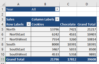
The formula =CUBEMEMBER(« offLine »; »[Products].[Product].[All].[Cookies] »)

searches for a single cell and returns the « Cookies » member, which has the caption we were looking for.
If you use the tuple: =CUBEMEMBER(« offLine »; « ([Stores].[Store].[All].[NorthEast],[Products].[All].[Cookies],[Years].[2008]) ») the result is 2008 (representing the cookie sales in the year 2008 in the NorthEast store).
If you use: =CUBEMEMBER(« offLine »; « ([Stores].[Group].[All].[North],[Stores].[Store].[All].[NorthEast] ») to find an empty intersection, you will get the #N/A error.
To display the word « total », enter: =CUBEMEMBER(« offLine », »[Products].[Product].[All] », »total »)
You can use the cell containing the formula to create cell captions. The actual content of the cell is more informative if it refers to the cells with the CUBEMEMBER() entries.
How to use the CUBEKPIMEMBER function in Excel
This function returns a Key Performance Indicator (KPI) property and displays the KPI name within the cell.
Syntax
CUBEKPIMEMBER(connection; kpi_name; kpi_property; caption)
Arguments
- connection (required): A string representing the name of the workbook connection to the cube. Upon entering the first quotation mark, existing context-sensitive data connections will be displayed.
- kpi_name (required): Specifies the name of the KPI in the cube.
- kpi_property (required): A KPI is composed of several components, specified using an integer (see below).
Integers for the Third Argument of the CUBEKPIMEMBER() Function
lnteger MDX expression Description
1 [KPIValue] Actual value
2 [KPIGoal] Target value
3 [KPIStatus] State of the KPI at a specific moment in time
4 [KPITrend] Measure of the value over time
5 [KPIWeight] Relative importance assigned to the KPI
6 [KPICurrentTimeMember] Temporal context for the KPI
Background
Error values and messages provide information regarding incorrect or missing entries:
- If the connection name is not a valid workbook connection, the CUBEKPIMEMBER() function returns the #NAME? error.
- If the OLAP server (or the offline cube) is unavailable, an error message will appear, but the content of the affected cell will not change.
- CUBEKPIMEMBER() returns the #N/A error value when kpi_name or kpi_property is invalid.
- CUBEKPIMEMBER() might return the #N/A error if the connection to the data source is interrupted and cannot be re-established.
You can combine CUBEKPIMEMBER() with CUBEVALUE(). To do so, specify CUBEKPIMEMBER() as the second argument or a reference for CUBEVALUE().
Example
In this example, a KPI named « average » is stored in the cube. This cube calculates the average of sales and the total number of sales as integers. Both values are also saved as measures in the cube but cannot be used to calculate fields in the PivotTable. The target value (goal) is $1,500. Figure below shows the example for cookies.
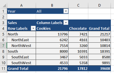
The formula =CUBEKPIMEMBER(« offline », »average »,1) displays the word « average ».

The formula =CUBEVALUE(« offline »,CUBEKPIMEMBER(« offline », »average »,1)) returns 1453 (the rounded average of all sales). In the second formula, you can also enter a reference to the cell containing the first formula as the second argument.
To get the target value of the average, use the formula =CUBEVALUE(« offline »,CUBEKPIMEMBER(« offline », »average »,2)). The value 2 in the last argument is important because, in this case, it indicates the target value.
You can use the cell containing the formula to create cell captions. The actual content of the cell becomes more informative when displayed using the CUBEVALUE() function.
How to use the GETPIVOTDATA function in Excel
This function retrieves data from a PivotTable report. You can use GETPIVOTDATA() to extract summarized data from a PivotTable report, provided that the summary data is visible within the report.
Syntax
GETPIVOTDATA(data_field; pivot_table; field1; item1; field2; item2; …)
Arguments
- data_field (required): The name, enclosed in quotation marks, of the data field that contains the data you wish to retrieve.
- pivot_table (required): A reference to a cell, cell range, or named cell range within a PivotTable report. This information helps to identify which PivotTable report contains the data you want.
- field1, item1, field2, item2, …: You must provide at least 1 and up to 14 pairs of field names and item names that describe the specific data you want to retrieve. These pairs can be in any order. Field names and item names (except for dates and numbers) must be enclosed in quotation marks. For OLAP (Online Analytical Processing) PivotTable reports, the items can include both the source name of the dimension and the source name of the item. An example of a field and item pair for an OLAP PivotTable might look like this: « [Product] », »[Product].[All Products].[Foods].[Baked Goods] ».
Background
The PivotTable in Excel is a powerful tool for data analysis. It allows you to sort data from a database and display summarized information. You can group, hide, filter, or evaluate your data without altering the raw data in your Excel table.
PivotTables are particularly effective because they enable you to change the data view in seconds, and they offer numerous layout options to create different perspectives of your data.
A PivotTable is most useful for databases and lists that contain similar elements that can be summarized based on various criteria. For instance, if five sales occurred in Seattle and three in Chicago, you can summarize these cities to view the total number of orders and the sum of sales. If there was only one sale per city, a summary wouldn’t be as useful, as you could retrieve that data directly from the database.
The GETPIVOTDATA() function allows you to retrieve data that has been summarized within a PivotTable report. You can reference any results from a PivotTable, whether it’s in the current workbook or another one.
Example
At the end of a business year, you want to create a PivotTable and then use the GETPIVOTDATA() function to identify the product with the highest sales.
First, you would select Data/Pivot Table And Pivot Chart Report to create a PivotTable (see Figure below).

The Figure below demonstrates how the GETPIVOTDATA() function can be used. A combo box allows the user to select a product, and the table below it displays the sales figures for each month for the selected product.
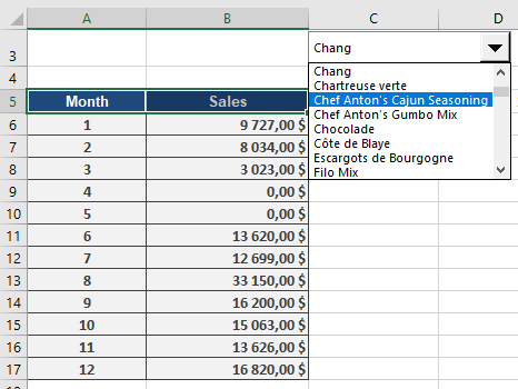
After selecting a product from the combo box, you want to display all sales for all countries that occurred within the year. Open a new worksheet and click on an empty cell. To test the GETPIVOTDATA() function, enter an equal sign (=) in the selected cell and then click any cell within the PivotTable you just created.
The GETPIVOTDATA() function will be applied automatically (see Figure below).

If you confirm the selected cell (cell B11 in the figure) by pressing the Enter key, the value $21,890 will appear in the worksheet (see Figure below).

Here are the arguments for the GETPIVOTDATA() function in this example: =GETPIVOTDATA(« Sales »,’Pivot from raw data’!$A$6, »Date »,1, »Product », »Camembert Pierrot »)
- « Sales »: This is the required data_field containing the data to be retrieved—in this case, the sales.
- ‘Pivot from original data’!$A$6: This is the pivot_table reference to cell A6 (or a cell range) within the PivotTable that contains the data you want to retrieve.
- « Date »,1: This is the first field1, item1 pair. « Date » is the field name, and 1 indicates January, meaning the sales for January are returned. 2 would indicate February, and so on.
- « Product », « Chai »: This is the first field2, item2 pair. « Product » is the field name, and « Chai » is the item name, meaning the sales for the product « Chai » are returned.
After familiarizing yourself with the GETPIVOTDATA() function, you decide to create a sales overview. Copy all item names from your original data list and paste them into the new worksheet (see Figure below).

Next, add a combo box to enable product selection from this list. If the « Developer » tab isn’t displayed, you’ll need to activate it.To add a combination field in Excel, right-click the menu bar and select « Form » to activate the « Form » toolbar. From the « Form » toolbar, drag a combination field onto the worksheet and open its properties. For « Input Range, » select the copied item names, and for « Cell Link, » assign an empty cell to the form.
When you click the arrow in the combo box, all item names will be available. In this example, the cell link is cell A2, and as a selection is made, the position of the selected entry in the list is displayed in this cell (see Figure below).
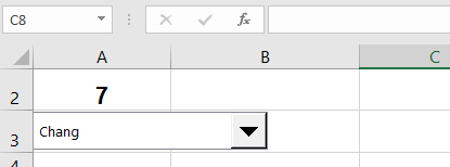
By using the INDEX() function, you can display the text value associated with the selection rather than just its position number. Click any empty cell in the worksheet and specify the arguments for the INDEX() function (see Figure below).
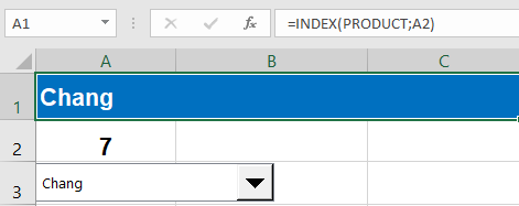
The following arguments are specified for the INDEX() function:
- array: This is the list of product names.
- row: A2 indicates the row or cell position to be returned.
- column: This argument doesn’t need to be specified because the row argument is used.
No matter which product you select in the combo box, the selection will be displayed as a label in cell A1.
To display the sales for each month, create a table with two columns: « Month » and « Sales. » Enter numbers 1 through 12 in the « Month » column, and then click the sales cell for month 1 (January). Enter an equal sign in this cell and click a cell under « January » in the PivotTable. Press the Enter key to confirm.
The Figure below shows the first entry in the sales cell for January.
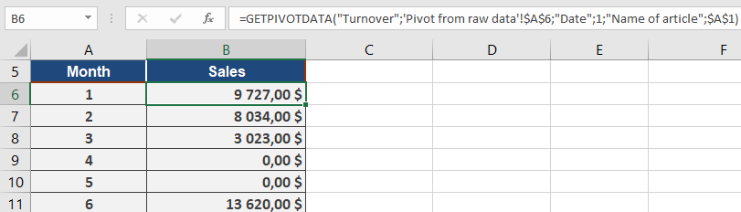
Now, you only need to modify the formula for the GETPIVOTDATA() function. The automatically generated formula displays the sales for January for the product « Alice Mutton. » Replace this with a reference to cell A1 to dynamically display the January sales for whatever product is selected in the combo box (see Figure below).

Finally, drag the formula in cell B6 down to the month of December to get the sales for all months, depending on the product selected in the combo box. The GETPIVOTDATA() function enables you to create neatly arranged summary tables.
How to use the DVARP function in Excel
This function calculates the variance of the entire population based on the numerical values in a column within a list or database that match the specified conditions.
Syntax
DVARP(database; field; criteria)
Arguments
- database (required): The cell range that constitutes your list or database.
- field (optional): Indicates which column the function will use.
- criteria (required): The cell range containing the field names and the filter criteria.
Background
The only difference between DVARP() and DVAR() is that the DVARP() function calculates the value based on the entire population.
Example
You have already calculated the variance for the sales of a product based on a sample using the DVAR() function. Now, you want to calculate the variance based on the entire population (see Figure below).

To put this into context, you also need to calculate the mean, as shown in Figure below.

The variance calculation based on a population meeting the criteria is $83,705.47. If you take the square root of this calculated variance, the result will be the standard deviation based on a population (refer to the DVAR() function, described earlier in this chapter).
How to use the DVAR function in Excel
This function estimates the variance of a sample based on the numerical values in a column within a list or database that match the specified conditions.
Syntax
DVAR(database; field; criteria)
Arguments
- database (required): The cell range that constitutes your list or database.
- field (optional): Indicates which column the function will use.
- criteria (required): The cell range containing the field names and the filter criteria.
Background
The most commonly used measures of spread in statistics are variance and standard deviation. The variance is calculated as the sum of the squared deviations of each value from the mean, divided by the number of values, with an adjustment made for the sample size.
Example
Since the sample variance measures the spread of data, it is frequently used in descriptive statistics.
Assume you are a wholesaler and want to use the DVAR() function to explain the variation in your sales orders. Let’s use the same example as for the DSTDEV() function. The objective here is to calculate the variance instead of the standard deviation, based on a sample with criteria defining the product and country/region selection (see Figure below).

To analyze the data, you will also need to calculate the mean, as shown in Figure below.

The result of the variance calculation, based on a sample and the set criteria, shows an average squared deviation of $90,680.52 from the arithmetic mean. If you take the square root of this variance, the result will be the standard deviation (as described earlier in this chapter, under the DSTDEV() function).
How to use the DSTDEVP function in Excel
This function calculates the standard deviation of an entire population based on the numerical values in a column within a list or database that match the specified criteria.
Syntax
DSTDEVP(database; field; criteria)
Arguments
- database (required): The cell range that constitutes your list or database.
- field (optional): Indicates which column the function will use.
- criteria (required): The cell range containing the field names and the filter criteria.
Background
The only difference between DSTDEVP() and DSTDEV() is that the DSTDEVP() calculation is based on the entire population and is not an estimate of the population value derived from a sample.
Example
As a wholesaler, you need to analyze your sales orders. You’ve already used the DSTDEV() function to calculate the standard deviation for a product’s sales based on a sample. Now, you want to calculate the standard deviation using the entire population.
Calculate the standard deviation based on the population of sales orders for a particular product in a specific country (see Figure below).

To effectively evaluate your findings, it’s also helpful to calculate the mean (see Figure below).

The calculation of the standard deviation based on the population and several criteria returns 289.32. This indicates that the sales of « Longlife Tofu » in the United States spread around the mean ($1,617.38) by $289.32.
How to use the DSTDEV function in Excel
This function estimates the standard deviation of a population based on a sample of data found in a column within a list or database that matches the specified conditions.
Syntax
DSTDEV(database; field; criteria)
Arguments
- database (required): The cell range that constitutes your list or database.
- field (optional): Indicates which column the function will use.
- criteria (required): The cell range containing the field names and the filter criteria.
Background
The standard deviation is a crucial measure of spread and quantifies the deviation from the arithmetic mean. It’s a measure of dispersion where a higher standard deviation indicates that the data is more spread out around the mean. The standard deviation is simply the square root of the variance.
Example
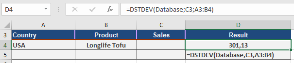
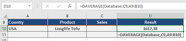
As a wholesaler, you’ve already analyzed your sales data using various functions. Now, you want to employ the DSTDEV() function to examine the dispersion of your sales. Specifically, you aim to understand how widely the sales orders for a particular product in a given country vary around the average order value.
In Figures below, the standard deviation is calculated for orders of « Longlife Tofu » in the United States. The result indicates a standard deviation of $301.13 around the mean of $1,617.38. Figure also illustrates the calculation of the average.
How to use the DPRODUCT function in Excel
This function multiplies the values in a specified column within a list or database that meet the defined conditions.
Syntax
DPRODUCT(database; field; criteria)
Arguments
- database (required): The cell range that constitutes your list or database.
- field (optional): Indicates which column the function will use.
- criteria (required): The cell range containing the field names and the filter criteria.
Background
Use the DPRODUCT() function to multiply values in a list based on specified criteria.
Example
The previous wholesaler example doesn’t offer suitable data to demonstrate this function effectively, so we’ll use a different scenario.
Assume you are a real estate agent and you’ve created a database for the apartments you are trying to sell (see Figure below).
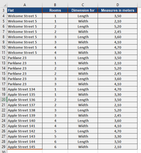
You have entered the dimensions of each room in the apartments and want to calculate the area of each room to provide this information to your customers. You can use the DPRODUCT() function to calculate the square meters. Figure below illustrates a possible solution.
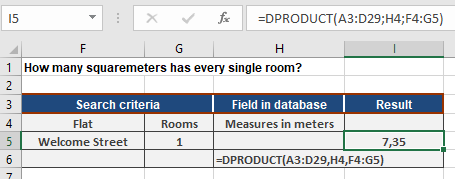
For this solution, the following arguments were used:
- Specify the cell range A3:D29 for the database argument.
- The street name and one of the rooms are used as the criteria fields (F4:G5).
- Specify cell H4 to identify the field argument.
The function returns 7.35 square meters for room 1 in the apartment on Welcome Street. If you change the value in cell G5 or the street name, you can calculate the area of other rooms in selected apartments.
How to use the DMIN function in Excel
This function returns the smallest numerical value from a specified column within a list or database, provided it matches the conditions you’ve set.
Syntax
DMIN(database; field; criteria)
Arguments
- database (required): This is the cell range that defines your list or database.
- field (optional): This indicates which column the function should use.
- criteria (required): This is the cell range containing the field names and the filter criteria you want to apply.
Background
You can use the DMIN() and DMAX() functions to find the smallest or largest value, respectively, in a database based on specific criteria. DMIN() will return a value from a database, such as the smallest sales figure for a product over the past five years.
Example
Your wholesale company is doing well with high sales, but you want to identify which product has the lowest sales. This insight could help you decide whether to modify the product or offer a different one. Specifically, you want to find the product with the lowest sales for a particular customer. The DMIN() function is perfect for this.
The DMIN() function will return the order value for the « Save-a-lot Markets » company (see Figure below). Since your database includes sales of $0, you’ll need to specify a criterion of >0 to exclude them.

DMIN() will then return the lowest sale of $1,020 for your customer, « Save-a-lot Markets. » You can also use the DGET() function to determine which product this specific sale was for. Figure below illustrates how to do this.

This approach allows you to analyze each customer and identify products with the smallest sales, helping you make informed decisions about adjusting your product line.