Votre panier est actuellement vide !
Catégorie : Excel function
How to use the BETA.DIST() function in Excel
This function returns values of the cumulative beta distribution, which is commonly used to analyze variance across samples (e.g., modeling proportions like daily computer usage time).
Syntax:
BETA.DIST(x; alpha; beta; cumulative; [A]; [B])Arguments:
- x (required): The value (between A and B) to evaluate.
- alpha (required): A shape parameter of the distribution.
- beta (required): A second shape parameter.
- cumulative (required): A logical value (TRUE = cumulative probability; FALSE = probability density).
- A (optional): Lower bound for x (default = 0).
- B (optional): Upper bound for x (default = 1).
Background
- The beta distribution models probabilities for variables bounded within a fixed interval (e.g., 0 to 1).
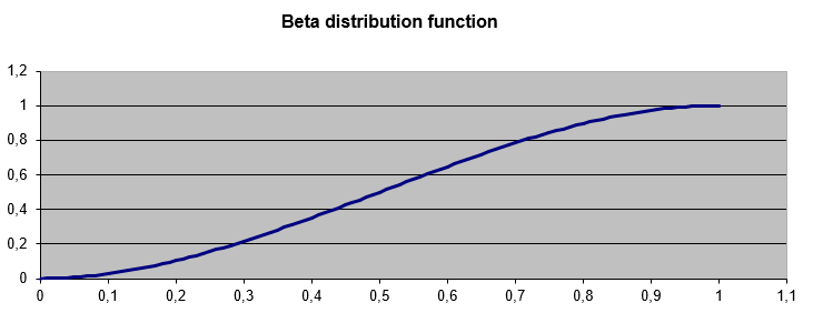
- alpha and beta control the distribution’s shape (see Figure below).
- If A and B are omitted, x must be between 0 and 1.
Example
Question:
What is the cumulative probability of x = 2 for a beta distribution with:- Shape parameters alpha = 8, beta = 10
- Bounds A = 1, B = 3?
Formula:
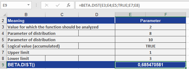
BETA.DIST(2, 8, 10, TRUE, 1, 3)Result: 0.68547 (see Figure below).
Interpretation:
There is a 68.547% probability that a randomly selected value from this distribution falls between 1 and 2.Key Notes
- Bounds: If A and B are specified, x must lie within [A, B].
- Cumulative vs. Density:
- TRUE: Returns the cumulative distribution (area under the curve up to x).
- FALSE: Returns the probability density at x.
- Applications: Useful for modeling proportions (e.g., task completion rates, survey responses).
How to use the AVERAGEIFS() function in Excel
This function calculates the average of cells that meet multiple specified criteria.
Syntax:
AVERAGEIFS(average_range; criteria_range1; criteria1; [criteria_range2; criteria2]; …)Arguments:
- average_range (required): The range of cells to average (must contain numeric values).
- criteria_range1 (required): The first range to evaluate against criteria1.
- criteria1 (required): The condition applied to criteria_range1 (number, expression, cell reference, or text).
- criteria_range2, criteria2, … (optional): Additional ranges and their associated criteria (up to 127 pairs).
Background
For general details on averages, see the AVERAGE() function description. Like AVERAGEIF(), AVERAGEIFS() measures central tendency but allows for multiple filtering conditions.
Example
Continuing the email marketing analysis from AVERAGEIF():
- You previously calculated the average click rate per mailing type.
- Now, you want to refine the analysis by excluding low click rates (<10,000) to avoid outlier distortion.
Formula Setup:
- average_range: D2:D30 (click rates to average).
- criteria_range1: C2:C30 (mailing types, e.g., « Software A »).
- criteria1: « Software A » (only include this mailing type).
- criteria_range2: D2:D30 (click rates again, for the second filter).
- criteria2: « >10000 » (only include clicks >10,000).
Result:
The average click rate for « Software A » mailings exceeding 10,000 clicks is 15,221.50 (as seen below).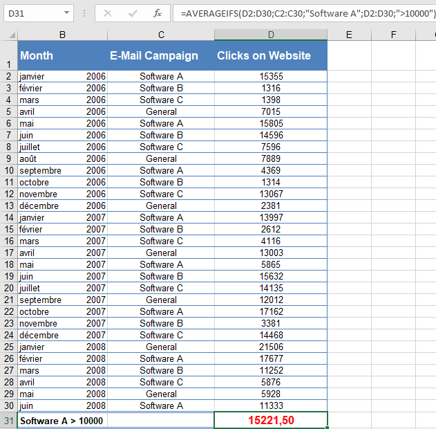
Key Notes
- Order Matters: The first argument is always the range to average, followed by criteria pairs.
- Flexibility: Supports numeric, text, and logical criteria (e.g., « >10000 », « =Completed »).
- Exclusion Logic: Unlike AVERAGEIF(), AVERAGEIFS() requires all criteria to be met for a cell to be included.
How to use the AVERAGEIF() function in Excel
This function calculates the average of all cells in a range that meet a specified criterion.
Syntax:
AVERAGEIF(range; criteria; [average_range])Arguments:
- range (required): The range of cells to evaluate against the criteria. These can include numbers, names, arrays, or references.
- criteria (required): The condition that determines which cells are averaged. It can be a number, expression, cell reference, or text.
- average_range (optional): The actual cells to average. If omitted, the function uses the range argument for both criteria evaluation and averaging.
Background:
For general information on averages, see the description of AVERAGE().The AVERAGEIF() function measures central tendency—the location of the center of a group of numbers in a statistical distribution. Unlike AVERAGE(), it allows you to apply a criterion that filters which values contribute to the mean.
The three most common measures of central tendency are:
- Average (Mean): The arithmetic mean of the distribution.
- Median: The middle value in a sorted list of numbers.
- Mode: The most frequently occurring value in a dataset.
In a symmetrical distribution, these measures are identical. In a skewed distribution, they may differ.
Example:
Your software company markets its products through email newsletters. To analyze engagement, you track the click rates on your website after each mailing over the past 30 months.Question: What is the average click rate after « Software B » mailings?
Using AVERAGEIF():
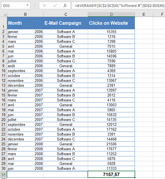
- Range (criteria evaluation): C2:C30 (contains mailing types, e.g., « Software B »).
- Criteria: « Software B » (only cells matching this label are considered).
- Average_range: D2:D30 (contains click rates to average).
Result: The average click rate after « Software B » mailings is 7,157.57 (see Figure below).
How to use the AVERAGEA() function in Excel
This function calculates the average of the values in an argument list. Unlike AVERAGE(), it includes not only numbers but also text and logical values (TRUE and FALSE) in the calculation.
Syntax:
AVERAGEA(value1; [value2] …)Arguments:
- value1(required) and value2 (optional): At least one and up to 255 arguments for which you want to calculate the average.
Background:
For more details on averages, refer to the definition of AVERAGE().The following rules apply to AVERAGEA():
- If an argument contains text (specified as an array or reference), it is evaluated as 0.
- Arguments containing TRUEevaluate as 1, and those containing FALSE evaluate as 0.
Note: If you do not want to include text values in the calculation, use the AVERAGE() function instead.
Example:
You work in the controlling department of a software company and create an Excel table containing sales data for the past twelve months.Since the list includes text and logical values, you calculate the average sales using AVERAGEA().
- In the first column, you enter the text « Closed » for February (see Figure below). Because AVERAGEA()automatically converts text to 0, all 12 values are summed, and the total is divided by 12. The result is $916.67.
- The second column contains TRUEinstead of « Closed. » This logical value is evaluated as 1. Again, all 12 values are summed, and the total is divided by 12. The result is $916.75.
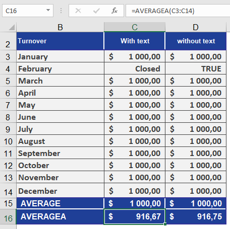
If you had used AVERAGE() instead, text values would be excluded—only 11 values would be summed, and the total divided by 11. In this case, the result would be $1,000.00.
How to use the AVERAGE() function in Excel
This function returns the average (arithmetic mean) of the arguments. To calculate the average, interval-scaled variables are summed and then divided by their count.
Syntax
AVERAGE(number1, number2, …)
Arguments
- number1 (required) and number2 (optional): At least one and up to 255 arguments (30 in Excel 2003 and earlier versions) for which you want to calculate the average.
Background
The arithmetic mean is the most well-known measure of central tendency and is widely used, even among non-statisticians. Because it incorporates all values in its calculation, it plays a key role in inferential statistics.
To compute the mean:
- Sum all values in a range.
- Divide the total by the number of values.
The arithmetic mean requires interval-scale data.
The combined mean of two datasets can also be derived from their individual arithmetic means.
Limitations
- Sensitivity to outliers: Extreme values significantly affect the mean since all data points are included.
- Potential misrepresentation: The mean may not align with actual observed values, especially in skewed distributions.
- Grouped data: For grouped or continuous variables, the arithmetic mean is only an estimate unless additional information about central tendency is available.
Applicability to Ordinal Data
Although the arithmetic mean typically requires metric-scale data, it can sometimes be applied to ordinal-scale data (e.g., customer satisfaction surveys) under certain conditions:
- The sample size is sufficiently large (n > 30).
- Data distribution approximates normality.
- A confidence interval is provided for the mean.
Comparison with Other Measures of Central Tendency
For datasets allowing arithmetic mean calculation, the mode and median can also be determined. The best measure depends on the context:
- Mean: Uses all data points but is sensitive to outliers.
- Median: Robust against outliers, ideal for skewed distributions.
- Mode: Best for categorical or highly clustered data.
Example
As a marketing manager for a software company, you need to calculate the average webpage visits in 2024 to identify high- and low-traffic areas.
Steps:
- Import website visit data into Excel.
- Use a PivotTable to organize visits by section (Products, Publications, Team, Training, Knowledge).
- Apply the AVERAGE() function to determine the mean visits per area.
Findings (see Figure below):
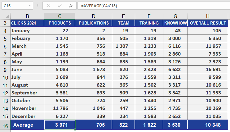
- The Products section has significantly more visits than Publications.
- The yearly average across all sections provides an overview of overall website activity.
- Comparing results with prior years enables trend analysis.
How to use the AVEDEV() function in Excel
This function returns the average of the absolute deviations of data points from their mean. The function calculates the arithmetic mean of the deviations of a data set based on the average, excluding the sign.
Syntax:
AVEDEV(number1, number2, …)AVEDEV() is a measure of the variance in a data set.
Arguments:
- number1(required) and number2 (optional): At least one and up to 255 arguments for which you want to calculate the absolute deviation. You can also use a single array or a reference to an array instead of arguments separated by commas.
Background:
To calculate the deviation of sales or, as in our example, the monthly website visits relative to the mean, use the AVEDEV() function.AVEDEV() is a measure of the variance in a data set.
In a sense, measures of dispersion serve as a quality criterion for the measure of central tendency. These measures indicate the accuracy of a measure of central tendency. Variance parameters refer to the difference between the following:
- Location values (range, quartile, or semi-quartile distance)
- Individual values and a mean (average linear deviation, variance, standard deviation)
Example:
The marketing department of a software company wants to analyse customer website visits. The visits to various website areas over the past 18 months are recorded in an Excel table (see table below).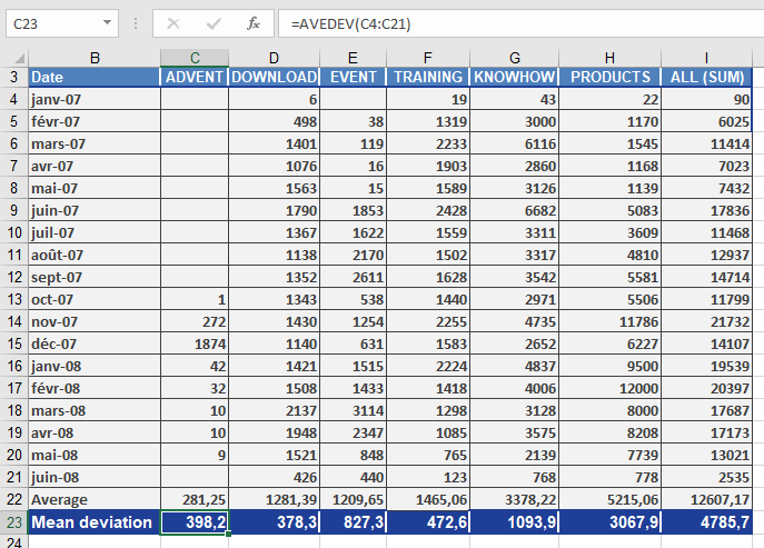
Since the average deviation refers to the mean values in the data sets, the marketing department calculates the mean value for each website area using the AVERAGE() function. Afterwards, they calculate the average deviation for each data set. The AVEDEV() function returns the results—the arithmetic mean of the deviation from the mean value.
Now, the mean values and average deviations can be compared and analyzed. The following conclusions can be drawn from this result:
The AVEDEV() function is a measure of the variance in a data set, where the variance parameters refer to the differences between individual values and mean values.
For example, the average deviation for the DOWNLOAD area is 378.3 per month. This means that, compared to the calculated mean value, the visits to the DOWNLOAD area vary by 378.3 each month.
How to use the CUBEVALUE function in Excel
This function returns the value of a member (cell) from a cube.
Syntax
CUBEVALUE(connection; member_expression1; member_expression2; …)
Arguments
- connection (required): A string representing the name of the workbook connection to the cube, enclosed in quotation marks. After you type the first quotation mark, existing context-sensitive data connections will be displayed.
- member_expression1 (required) and member_expression2 (optional): You must provide at least one and up to 255 expressions that define the position of a member in the cube based on a Multidimensional Expression (MDX). The expression can be entered directly or referenced from a cell. Tuples can also be used in expressions. Alternatively, a member_expression can be a set defined with the CUBESET() function. If no measure is specified in a member_expression, the default measure for that cube is used. Because this argument can be repeated, you can define intersections. You can also use tuples.
Background
When you use CUBEVALUE() as an argument for another cube function, the MDX expression (rather than the displayed value) is used in the argument.
Error values and messages provide information about incorrect or missing entries:
- If the connection name is not a valid workbook connection, the CUBEVALUE() function returns the #NAME? error.
- If the OLAP server (or the offline cube) is unavailable, an error message will appear, but the content of the affected cell will not change.
- If at least one member within the arguments or the tuple is invalid, the CUBEVALUE() function returns the #VALUE!.
- If a member_expression is longer than 255 characters, the CUBEVALUE() function returns the #VALUE!.
- CUBEVALUE() returns the #N/A error when:
- The member_expression syntax is incorrect.
- The member specified in the MDX query does not exist in the cube.
- The tuple is invalid because there is no intersection for the specified values.
- The set contains at least one member with a different dimension from the other members.
- CUBEVALUE() might also return the #N/A error when the connection to the data source is interrupted and cannot be re-established.
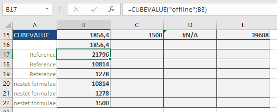
The formula: =CUBEVALUE(« offLine », »[Measures].[GrossSales] », »[Stores].[Store].[All].[NorthEast] », »[Years].[Year].[All].[2009] », »[Products].[Product].[All].[Cookies] ») calculates the gross sales for cookies in the « NorthEast » store in the year 2009, which is $1,856.40. You will get the same result if you use a tuple (where the arguments of the previous formula are enclosed in parentheses): =CUBEVALUE(« offline », »([Measures].[GrossSales],[Stores].[Store].[All].[NorthEast],[Years].[Year].[All].[2009],[Products].[Product].[All].[Cookies]) »)
If you enter the formula =CUBEMEMBER(« offLine », »[Products].[Product].[All].[Cookies] ») in cell B3, then the formula =CUBEVALUE(« offline »,B3) returns the total sales for cookies: $21,796.
You can also use examples from the CUBEKPIMEMBER() function. For instance, the formula: =CUBEVALUE(« offline »,CUBERANKEDMEMBER(« offline »,CUBESET(« offline », »[Stores].[Store].Children », »all store sales »,2; »[Measures].[Sale] »),1)) returns $10,814 for the total sales of the best-performing store (« NorthEast »).
How to use the CUBESETCOUNT function in Excel
This function returns the number of members in a set.
Syntax
CUBESETCOUNT(set)
Argument
- set (required): A set defined using the CUBESET() function, or a reference to a cell that contains members of the cube.
Background
The result of this function is an integer. If the argument causes an error, that error will also be returned as the result.
Example
If you reference a cell in the CUBESETCOUNT() function that returns the sorted set of stores, such as with the formula:
=CUBESET(« offline », »[Stores].[Store Name].Children »; « all sales »;2; »[Measures].[Sale] »)

the result will be 4. You’ll get the same result if you pass this entire formula as an argument directly to CUBESETCOUNT(). Note that the keyword Children is not context-sensitive.
How to use the CUBESET function in Excel
This function returns a calculated set of members by sending a set expression to the cube on the server, which then creates and returns that set to Excel. Note that the displayed content of the cell and its actual value will differ.
Syntax
CUBESET(connection; set_expression; caption; sort_order; sort_by)
Arguments
- connection (required): A string that specifies the name of the workbook connection to the cube, enclosed in quotation marks. As you type the first quotation mark, existing context-sensitive data connections will be displayed.
- set_expression (required): Defines the number of elements in the cube based on a Multidimensional Expression (MDX). You can enter the expression directly or reference a cell containing the expression. Tuples can also be used in expressions.
- caption (optional): A string to be displayed in the cell instead of the member’s caption from the cube. If a tuple is used, the function returns the caption of the last member in the tuple.
- sort_order (optional): This integer value determines the type of sorting and affects how the fifth argument, sort_by, is treated (see Table 1). The available options are context-sensitive.
Table 1. Integers for the Fourth Argument of the CUBESET() Function
lnteger Description lmpact on the Fifth Argument 0
Leaves the set in the existing order in the cube
Ignored
1
Sorts the set in ascending order by
sort_by
Required
2
Sorts the set in descending order by
sort_by
Required
3
Sorts the set in ascending alphabetical order
Ignored
4
Sorts the set in descending alphabetical order
Ignored
5
Sorts the set in natural ascending order
Ignored
6
Sorts the set in natural descending order
Ignored
The default value for the fourth argument is 0. Alphabetical sorting for a set of tuples is based on the last element in the tuple. You can find more information about different sort orders in the SQL Analysis Services Help documentation.
- sort_by (optional): This argument depends on the fourth argument (sort_order) and defines the values within the set that will be sorted. If sort_by is not provided but sort_order requires it, the function returns the #VALUE! error.
Background
When you use CUBESET() as an argument for another cube function, the set itself (not its displayed value) is used in the argument.
Error values and messages provide information about incorrect or missing entries:
- If the connection name is not a valid workbook connection, the CUBESET() function returns the #NAME? error.
- If the OLAP server (or the offline cube) is unavailable, an error message will appear, but the content of the affected cell will not change.
- If set_expression is longer than 255 characters, the CUBESET() function returns the #VALUE! error.
- CUBESET() returns the #N/A error when:
- The set_expression syntax is incorrect.
- The set specified in the MDX query does not exist in the cube.
- The set contains at least one member with a different dimension from the other members.
- CUBESET() might also return the #N/A error when the connection to the data source is interrupted and cannot be re-established.
Example
The formula =CUBESET(« offline », »[Stores].[Store Name].Children », « all sales »,2, »[Measures].[Sale] ») returns the sorted set of all stores based on their sales (across all products and years). The store with the largest sale will be listed first.
You can use the cell containing the formula to create cell labels. The actual content of the cell becomes more informative when it refers to cells containing CUBESET() entries.

How to use the CUBERANKEDMEMBER function in Excel
This function returns the n-th member in a set.
Syntax
CUBERANKEDMEMBER(connection; set_expression; rank; caption)
Arguments
- connection (required): A string representing the name of the workbook connection to the cube. After you type the first quotation mark, existing context-sensitive data connections are displayed.
- set_expression (required): Defines the number of members in the cube based on a Multidimensional Expression (MDX). The expression can be entered directly or referenced from a cell. Tuples can also be used in expressions.
- rank (required): An integer indicating the position of a member within the set.
- caption (required): A string to be displayed in the cell instead of the member’s caption from the cube. If a tuple is used, the function returns the caption of the last member in the tuple.
Background
Error values and messages provide information about incorrect or missing entries:
- If the connection name is not a valid workbook connection, the CUBERANKEDMEMBER() function returns the #NAME? error.
- If the OLAP server (or the offline cube) is not available, an error message will appear, but the content of the affected cell will not change.
- If set_expression is longer than 255 characters, the CUBERANKEDMEMBER() function returns the #VALUE! error.
- CUBERANKEDMEMBER() returns the #N/A error when:
- The set_expression syntax is incorrect.
- The set specified in the MDX query does not exist in the cube.
- CUBERANKEDMEMBER() might also return the #N/A error when the connection to the data source is interrupted and cannot be re-established.
Example
If you reference a cell in the formula =CUBERANKEDMEMBER(« offline »,B9,1) that returns the store set with =CUBESET(« offline », »[Stores].[Store].Children », « all store sales »,2, »[Measures].[Sale] »), the result is NorthEast. This store has the most sales for all products and in all years.
The nested formula =CUBERANKEDMEMBER(« offLine »,CUBESET(« offLine », »([Stores].[Store].[All].[NorthEast], [Years].Children) », »all sales »,2; »[Measures].[Sales] »),3) calculates the year with the least sales for this store (position 3): 2011.
