Votre panier est actuellement vide !
Catégorie : Excel function
How to use the BESSELJ() function in Excel
This function returns the Bessel function of the first kind, Jₙ(x).
Syntax
BESSELJ(x ; n)Arguments
- x (required)
The value at which to evaluate the function:- Must be a real number
- Valid range: approximately -1.34×10⁸ to +1.34×10⁸ (range varies with order n)
- n (required)
The order of the Bessel function:- Must be positive
- Non-integer values are truncated (decimal places ignored)
Background
The Bessel function Jₙ(x) is a solution to Bessel’s differential equation:x²y » + xy’ + (x² – n²)y = 0
or
y » + (1/x)y’ + (1 – n²/x²)y = 0
For real ν, the function can be calculated using:

where Γ(y) is the gamma function.
Example
Due to the specialized nature of Bessel functions, this example focuses on their graphical representation (see Figures below).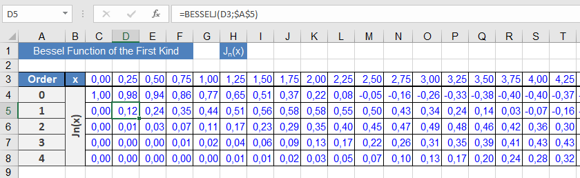
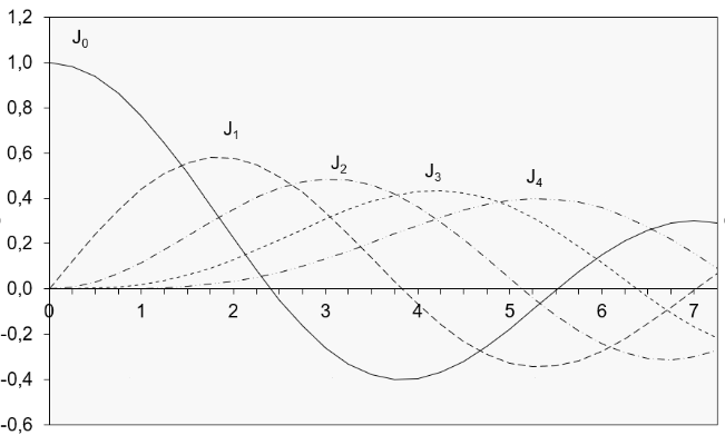
Implementation notes:
- The sample worksheet calculates Jₙ(x) for orders 0 through 4
- Results are displayed in the graph shown in Figure above
- The oscillatory behavior characteristic of Jₙ(x) is clearly visible
Key Properties
- Oscillates with decreasing amplitude as x increases
- Jₙ(-x) = (-1)ⁿJₙ(x)
- For integer n, Jₙ and J₋ₙ are linearly dependent
- Satisfies various recurrence relations
Technical Applications
- Cylindrical wave propagation
- Heat conduction in circular geometries
- Solutions to Laplace’s equation in polar coordinates
- Modeling of drumhead vibrations
Computation Notes
- Calculated via power series expansion
- Accuracy depends on argument range and order
- Higher orders require more terms for convergence
- x (required)
How to use the BESSELI() function in Excel
This function returns the modified Bessel function of the first kind, Iₙ(x), which corresponds to the Bessel function Jₙ evaluated for purely imaginary arguments.
Syntax
BESSELI(x ; n)Arguments
- x (required)
The value at which to evaluate the function:- Must be a real number
- Valid range: approximately ±700 (varies with order n)
- n (required)
The order of the Bessel function:- Must be a positive integer
- Non-integer values are truncated (not rounded)
Background
Iₙ(x), like Kₙ(x), belongs to the modified Bessel functions that exhibit exponential growth or decay, unlike the oscillatory behavior of standard Bessel functions Jₙ(x) and Yₙ(x). Iₙ(x) is the solution to the modified Bessel’s differential equation:x²y » + xy’ – (x² + n²)y = 0
or
y » + (1/x)y’ – (1 + n²/x²)y = 0
The modified Bessel function of the first kind can be represented as a loop integral of order n. For real ν, it can be calculated using:
I_ν(x) = (1/π) ∫[0 to π] e^{x cosθ}cos(νθ) dθ
where Γ(y) is the gamma function.
Example
Working with Bessel functions requires specialized domain knowledge. This example focuses on mathematical properties and their graphical representation (see Figure below).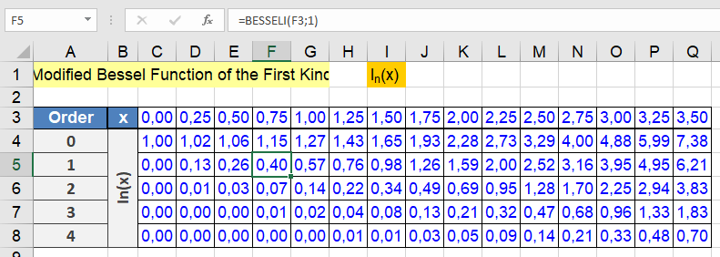
Implementation notes:
- Cell A3 contains the reference label « Order »
- Cells C4:Q8 contain BESSELI() formulas
- Row 3 contains x-values (first argument)
- Column A contains order values (second argument)
- Example formula in C4:
=BESSELI(C$3,$A4)
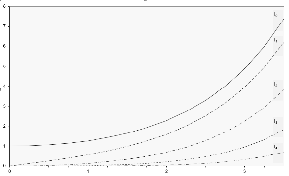
The data range C3:Q8 generates the graph in Figure below, showing the characteristic exponential growth of Iₙ(x), which produces large values even at small x.
Key Properties
- Exhibits monotonic exponential growth
- Iₙ(0) = 0 for n > 0
- Iₙ(-x) = (-1)ⁿIₙ(x)
- Recurrence relations connect functions of different orders
Technical Applications
- Electromagnetic wave propagation
- Heat conduction in cylindrical systems
- Quantum mechanical potential problems
- Fluid dynamics in porous media
- x (required)
How to use the BIN2HEX() function in Excel
This function converts a binary number into a hexadecimal number.
Syntax
BIN2HEX(number; [places])Arguments
- number(required) – The binary number to be converted:
- Maximum of 10 digits
- Uses two’s complement notation (see « Two’s Complement » section)
- Negative values return a 10-digit hexadecimal number
- places(optional) – Specifies the number of digits to display:
- Adds leading zeros if needed
- If omitted, displays only necessary digits
- Decimal places are ignored
Background
For comprehensive information about number systems and conversion methods, refer to the « Number Systems » section in the function introduction.Examples
The following examples demonstrate the BIN2HEX() function:- =BIN2HEX(000000001)returns 1
- =BIN2HEX(1110,4)returns 000E
- =BIN2HEX(000001010)returns 0A

Additional Resources
More examples can be found in the BIN2DEC() function documentation.Key Features
- Handles both positive and negative binary numbers
- Optional places parameter for formatting
- Automatic sign detection through two’s complement
- 10-digit binary input limit
- Returns full 10-digit hex for negative numbers regardless of places parameter
- number(required) – The binary number to be converted:
How to use the BIN2DEC() function in Excel
This function converts a binary number into a decimal number.
Syntax
BIN2DEC(number)Argument
- number(required) – The binary number to be converted, which must:
- Be in two’s complement notation
- Contain no more than 10 digits
Background
For detailed information about number systems and two’s complement notation, refer to the « Number Systems » section in the introduction to these functions.Examples
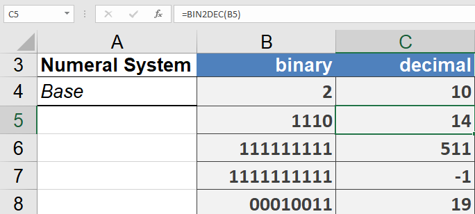
The following examples demonstrate the BIN2DEC() function:- =BIN2DEC(1110)returns 14
- =BIN2DEC(111111111)returns 511
- =BIN2DEC(1111111111)returns -1 (demonstrating two’s complement representation)
- =BIN2DEC(1111111110)returns -2
Key Notes
- The function handles both positive and negative numbers through two’s complement representation
- The 10-digit limit is important as it determines the range of numbers that can be represented
- For positive numbers, the conversion is straightforward binary-to-decimal
- For negative numbers (indicated by a leading 1 in two’s complement), the function properly interprets the two’s complement notation
- number(required) – The binary number to be converted, which must:
How to use the TANH() function in Excel
This function returns the hyperbolic tangent of a number.
Syntax
TANH(number)Argument
- number (required) – Any real number.
Background
- The hyperbolic tangent is part of the hyperbolic functions, which (like trigonometric functions) are defined for all real and complex numbers. However, Excel only supports real-number arguments for hyperbolic functions.
- The formula for the hyperbolic tangent is:
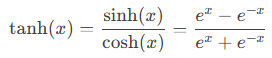
The last term highlights its similarity to trigonometric functions.
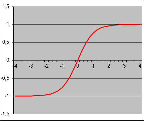
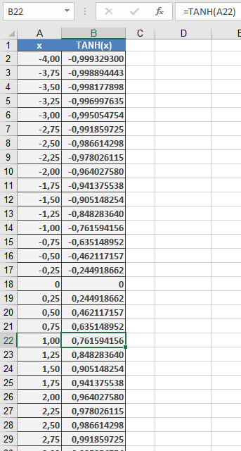
- The hyperbolic tangent is widely used in engineering and natural sciences for research and development (see Figure below).
Missing Cotangent Functions
- Unlike trigonometric functions (sin, cos, tan, cot), Excel does not include built-in hyperbolic cotangent (COTH) or trigonometric cotangent (COT) functions.
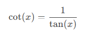
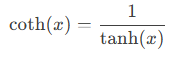
- However, both can be derived as reciprocals of their tangent counterparts:
- Trigonometric cotangent:
-
- Hyperbolic cotangent:
- Workaround in Excel:
Instead of =COTH(A1) (which does not exist), use:
=1/TANH(A1)
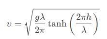
Example: Wave Propagation Speed Calculation
Application:
The hyperbolic tangent is used to calculate the propagation speed (υυ) of waves, given:- Gravity acceleration (gg) in [m/s²],
- Wave length (λλ) in [m],
- Water depth (hh) in [m].
Formula:
Approximations for Shallow/Deep Water:
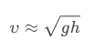
- Shallow water (h≪λh≪λ):
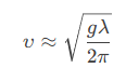
- Deep water (h≫λh≫λ):
Additional Examples
=TANH(0) // Returns 0
=TANH(1) // Returns 0.761594156
=TANH(-1) // Returns -0.76159416
=TANH(10) // Returns 1 (approaches asymptotically)
=TANH(-10) // Returns -1 (approaches asymptotically)
Key Properties:
- Output ranges between -1 and 1.
- For large positive/negative inputs, TANH() approaches ±1.
How to use the TAN() function in Excel
This function returns the tangent of an angle.
Syntax
TAN(number)Argument
- number (required) – The angle in radians for which you want the tangent.
Background
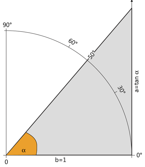
- In a right triangle, the tangent of an angle is the ratio of the length of the opposite side to the length of the adjacent side.
- The TAN() function requires the angle to be in radians. If the angle is given in degrees, convert it by multiplying by PI()/180 or using the RADIANS() function.
- For an angle α in a unit circle (r=1):
- As α increases from 0° to 90°, the tangent increases from 00 to +∞+∞ (see Figure below).
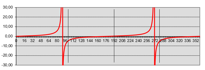
- In a coordinate system, plotting the angle αα on the x-axis and tan(α)tan(α) on the y-axis produces the curve shown in Figure below.
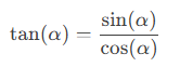
Tangent Relationship with Sine and Cosine:

Practical Application (Slope Calculation):
- The tangent describes the relationship between the gradient angle and the slope of a line.
- Example: A road with a gradient angle of 12°12° has a slope of tan(12°)≈0.21tan(12°)≈0.21, often displayed as 21% (21 meters elevation per 100 meters horizontally).
- Note: The tangent is undefined at 90° and −90° (vertical slope).
Example:
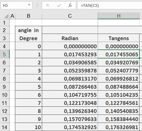
Key Steps:
- Convert degrees to radians (RADIANS()).
- Calculate tangent (TAN()).
- Multiply by distance and round (ROUND()).
- Add observer’s eye level.
How to use the SUMXMY2() function in Excel
This function returns the sum of squares of differences of corresponding values in two arrays.
Syntax
SUMXMY2(array_x; array_y)Arguments
- array_x(required) – The first array or range of values.
- array_y(required) – The second array or range of values.
Background
- The arguments should be numbers, names, arrays, or references containing numbers.
- If an array or a reference argument contains text, logical values, or empty cells, those values are ignored. However, cells with the value zero are included.
- If array_xand array_y have a different number of values, the SUMXMY2() function returns the #N/A
The equation for the sum of squared differences is:
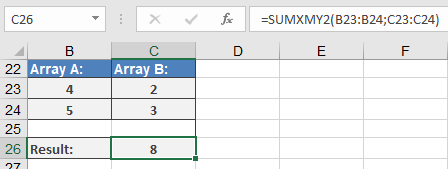
Σ(x – y)²The solution of this equation is built for the example (see Figure below) as follows:
- In two specified ranges:
- Range A:4, 5
- Range B:2, 3
The corresponding values are subtracted:
- First pair: 4 – 2 = 2
- Second pair: 5 – 3 = 2
- The differences are squared and summed (see Figure 16-37):
- 2² + 2² = 4 + 4 = 8
How to use the SUMX2PY2() function in Excel
This function returns the sum of the sum of squares of corresponding values in two arrays. The sum of the sum of squares is a common term in many statistical calculations.
Syntax
SUMX2PY2(array_x; array_y)Arguments
- array_x(required) – The first array or range of values.
- array_y(required) – The second array or range of values.
Background
- The arguments should be numbers, names, arrays, or references containing numbers.
- If an array or a reference argument contains text, logical values, or empty cells, those values are ignored. However, cells with the value zero are included.
- If array_xand array_y have a different number of values, the SUMX2PY2() function returns the #N/A
The equation for the sum of the sum of squares is:
Σ(x² + y²)EXAMPLE
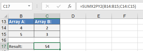
The solution of this equation is built for the example (see Figure below) as follows:
- In two specified ranges:
- Range A:4, 5
- Range B:2, 3
The square of each value is calculated:
- Range A:16, 25
- Range B:4, 9
- The squares of all values in each range are summed:
- Range A:16 + 25 = 41
- Range B:4 + 9 = 13
- The sums are added together (see Figure 16-36):
41 + 13 = 54
How to use the SUMX2MY2() function in Excel
This function returns the sum of the difference of squares of corresponding values in two arrays .
Syntax
SUMX2MY2(array_x; array_y)
Arguments
- array_x (required) – The first array or range of values.
- array_y (required) – The second array or range of values.
Background
- The arguments should be numbers or names, arrays, or references containing numbers.
- If an array or reference argument contains text, logical values, or empty cells, those values are ignored. However, cells with the value zero are included.
- If array_x and array_y have a different number of values, the SUMX2MY2() function returns the #N/A error.
The equation for the sum of the difference of squares is:
Σ(x² – y²)EXAMPLE
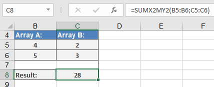
The solution for this equation is built for the example (see Figure below) as follows:
- In two specified ranges:
- Range A: 4, 5
- Range B: 2, 3
The square of each value is calculated:
-
- Range A: 16, 25
- Range B: 4, 9
- The squared values are summed:
- Range A: 16 + 25 = 41
- Range B: 4 + 9 = 13
- The sums are subtracted (see Figure below):
41 – 13 = 28
How to use the SUMPRODUCT() function in Excel
Its multiplies corresponding components in given arrays and returns the sum of those products.
Syntax:
SUMPRODUCT(array1; [array2]; [array3]; …)Arguments:
Argument Description array1 (required) First array of values array2 (required) Second array of values array3,… (optional) Additional arrays (up to 255 in modern Excel) Key Features:
- Calculation Method:
- Performs element-wise multiplication (a₁×b₁, a₂×b₂,…)
- Sums all resulting products
- Formula: Σ(array1[i] × array2[i] × …)
- Requirements:
- All arrays must have identical dimensions
- Non-numeric values are treated as zero
- Returns #VALUE! if arrays have different sizes
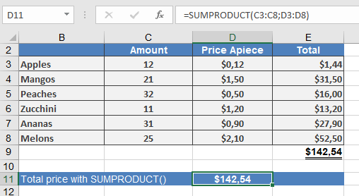
Example: Product Price Calculation
Common Errors:
- #VALUE!: Array size mismatch
- Incorrect results: Hidden text values treated as zero
Related Functions:
- SUM(): Simple addition
- MMULT(): Matrix multiplication
- SUMIFS(): Conditional sum with multiple criteria
Note:
While originally designed for simple array multiplication, SUMPRODUCT has become a powerful tool for complex array operations in Excel.- Calculation Method: