Catégorie : Excel function

Its adds all numbers in a range that meet multiple specified criteria (introduced in Excel).

Syntax:
SUMIFS(sum_range; criteria_range1; criteria1; [criteria_range2; criteria2]; …)

Arguments:

Argument	Description
sum_range (required)	Range of cells to sum
criteria_range1 (required)	First range to evaluate
criteria1 (required)	First condition (number, expression, or text)
criteria_range2, criteria2,… (optional)	Additional ranges/criteria (up to 127 pairs)

Key Features:

1. Criteria Formats:
   • Number: 32
   • Comparison: « >32 »
   • Text: « apples » (exact) or « a* » (wildcard)
   • Cell reference: I7
2. Behavior:
   • All criteria must be met for inclusion
   • Case-insensitive text matching
   • Supports wildcards (*, ?)
   • More flexible than SUMIF() (which allows only 1 criterion)

Example: Sales by Month, Company & Product
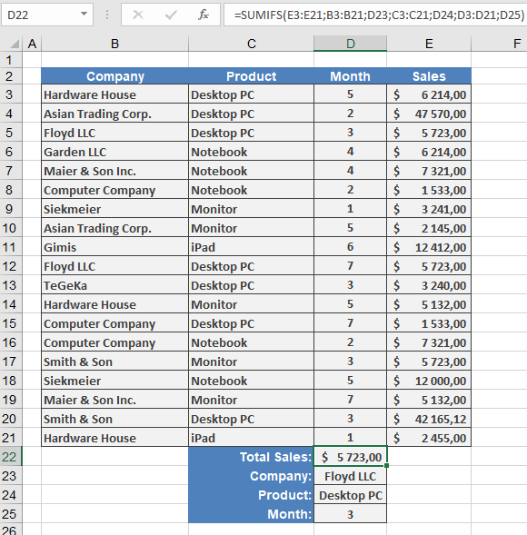
Scenario: Sum sales for « Contoso, Ltd. » purchasing « Desktop PC » in « Month 3 »

Data Structure:

B3:B21 = Companies 

C3:C21 = Products 

D3:D21 = Months 

E3:E21 = Sales amounts 

I7 = « Contoso, Ltd. » 

I8 = « Desktop PC » 

I9 = 3 (Month) 

Formula:

=SUMIFS(E3:E21; B3:B21; I7; C3:C21; I8; D3:D21; I9)

Breakdown:

1. Sums values in E3:E21 where:
   • B3:B21 matches « Contoso, Ltd. »
   • C3:C21 matches « Desktop PC »
   • D3:D21 equals 3
2. Returns $5,723

Practical Notes:

• Order of criteria doesn’t affect results
• Ranges must be same size (but non-contiguous)
• For single-criterion sums, SUMIF() is simpler

Common Errors:

• #VALUE!: Mismatched range sizes
• Unexpected results: Verify criteria syntax (e.g., « > »&I9 for dynamic comparisons)

Related Functions:

• SUMIF(): Single-criterion version
• COUNTIFS(): Count with multiple criteria
• AVERAGEIFS(): Average with multiple criteria

Its adds all values in a range that meet specified criteria.

Syntax:
SUMIF(range; criteria; [sum_range])

Arguments:

Argument	Description
range (required)	Range of cells to evaluate against the criteria
criteria (required)	Condition that determines which cells to add (number, expression, or text)
sum_range (optional)	Actual cells to sum (if omitted, uses ‘range’ for summing)

Key Features:

1. Criteria Formats:
   • Number: 32
   • Comparison: « >32 »
   • Text: « apples » (exact match) or « a* » (wildcard match)
   • Cell reference: A9
2. Behavior:
   • Case-insensitive for text criteria
   • Supports wildcards (* for multiple characters, ? for single character)
   • Omitting sum_range sums the criteria range itself

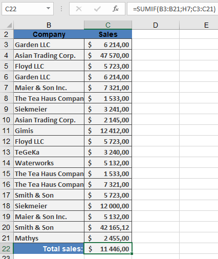
Example: Sales by Representative

Notes:

• For multiple criteria, use SUMIFS()
• Related functions:
  • COUNTIF(): Count cells meeting criteria
  • AVERAGEIF(): Average cells meeting criteria

Common Errors:

• #VALUE!: Incompatible criteria type
• Incorrect sums: Verify ranges are same size when using sum_range

Its returns the sum of all specified numbers or ranges.

Syntax:
SUM(number1; [number2]; …)

Arguments:

Argument	Description
number1	Required. First number or range to sum
number2,…	Optional. Additional values to sum (1-254 total)

Key Features:

1. Input Flexibility:
   • Accepts individual numbers (=SUM(1,2,3))
   • Accepts cell ranges (=SUM(A1:A10))
   • Accepts mixed arguments (=SUM(A1:A5,10,B2:B4))
2. Automatic Handling:
   • Ignores empty cells, text, and logical values in ranges
   • Converts numeric text (« 12 ») to numbers
   • Treats TRUE as 1 and FALSE as 0
   • Returns errors if arguments contain error values

Technical Specifications:

• Maximum 255 arguments
• Works with numbers up to 15-digit precision
• Processes up to 32,767 characters in formula text

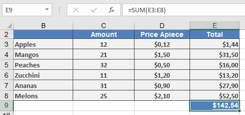
Examples:

Best Practices:

1. Use the Alt+= shortcut for quick sum insertion
2. For conditional sums, consider:
   • SUMIF() for single criteria
   • SUMIFS() for multiple criteria
3. To sum only visible cells, use SUBTOTAL(9, range)

Common Errors:

Error	Cause	Solution
#VALUE!	Non-numeric text argument	Verify data types
#REF!	Invalid reference	Check range addresses
#NAME?	Misspelled function	Correct to « SUM »

Version Notes:

• Behavior consistent across all Excel versions
• Argument limit increased from 30 to 255 in Excel 2007

Related Functions:

• SUBTOTAL(): Ignore filtered/hidden rows
• SUMIF(): Conditional summation
• SUMPRODUCT(): Sum of products

This function returns a subtotal for a range of data, typically used in lists or databases. While the Data > Subtotal command is often easier for creating subtotals, the SUBTOTAL() function allows for post-creation modifications.

Syntax:
SUBTOTAL(function_num; ref1; [ref2]; …)

Arguments:

1. function_num (required)
   • A number between 1–11 (includes hidden rows) or 101–111 (excludes hidden rows) that specifies the calculation method.

Table 1: Function Codes

Code (Includes Hidden)	Code (Excludes Hidden)	Function
1	101	AVERAGE()
2	102	COUNT()
3	103	COUNTA()
4	104	MAX()
5	105	MIN()
6	106	PRODUCT()
7	107	STDEV()
8	108	STDEVP()
9	109	SUM()
10	110	VAR()
11	111	VARP()

1. ref1, ref2, …
   • ref1 (required): The range to subtotal.
   • ref2 (optional): Additional ranges (up to 254 total).

Key Features:

1. Filters & Hidden Rows:
   • Codes 1–11 include rows hidden manually (Format > Hide).
   • Codes 101–111 exclude manually hidden rows.
   • Always ignores rows filtered out (regardless of code).
2. Nested Subtotals:
   • Automatically skips other SUBTOTAL() results within the range to avoid double-counting.
3. Limitations:
   • Fails with 3D references (#VALUE! error).
   • Designed for vertical ranges (columns). Hiding columns in horizontal ranges (e.g., =SUBTOTAL(109,B2:G2)) has no effect.

Example: Filtered Sum

Scenario: Calculate total sales for Michigan after filtering.

1. Original Data (C2:C8):

=SUBTOTAL(9, C2:C8)  // Sum all visible rows (includes hidden)

or

=SUBTOTAL(109, C2:C8)  // Sum only non-hidden rows

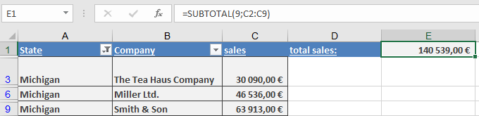
1. After Filtering (Michigan):
   • The result automatically updates to exclude filtered-out states.

Note: For dynamic reports, combine with Excel’s Filter or Table features.

This function returns the square root of a number multiplied by π (pi).

Syntax:
SQRTPI(number)

Argument:

• number(required) – The positive number to be multiplied by π before taking the square root.

Background:

• Calculates √(number × π)
• Only accepts positive numbers
• Returns #NUM!error for negative inputs

Examples:

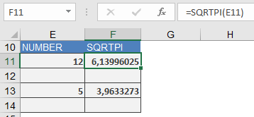
• =SQRTPI(12)returns 6,13996025
  (√(12×π) ≈ √37.6991118 ≈ 6.13996025)
• =SQRTPI(5)returns 3,9633273
  (√(5×π) ≈ √15.7079633 ≈ 3.9633273)

Key Notes:

1. Equivalent to =SQRT(number*PI())
2. Useful for circular calculations (e.g., wave functions, geometry)
3. More efficient than separate multiplication and root operations

Common Applications:

• Physics (wave equations)
• Engineering (structural calculations)
• Geometry (circle-related formulas)

This function returns the square root of a number.

Syntax:
SQRT(number)

Argument:

• number(required) – The number for which you want to calculate the square root.

Background:
The root function is the inverse of exponentiation.

• The base (b) is called the radicand
• x represents the root order
• When the root order is 2, it is called a square root

Note:
The SQRT() function only returns the square root of positive numbers. If the input number is negative, the function returns a #NUM! error.

Example:
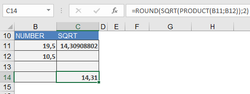
Calculate the dimensions of a square building lot with the same area as a rectangular lot measuring 19.5 × 10.5 meters.

1. Rounded result:
   =ROUND(SQRT(PRODUCT(B11;B12)),2)
   Returns: 14,31meters

Calculation steps explained:

1. Calculate the area (product of dimensions):
   =PRODUCT(19.5,10.5)
2. Extract the square root of the area:
   =SQRT(PRODUCT(19.5,10.5))
3. Round the result to 2 decimal places:
   =ROUND(SQRT(…),2)

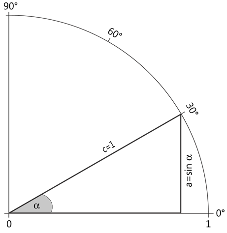
Its returns the trigonometric sine of an angle. The sine represents the ratio of the length of the opposite side to the hypotenuse in a right-angled triangle.

Syntax:
SIN(number)

Argument:

Argument	Description
number (required)	The angle in radians for which you want to calculate the sine

Key Concepts:

1. Right Triangle Relationship: In a right triangle, sin(α) = opposite side / hypotenuse
2. Unit Circle Properties:
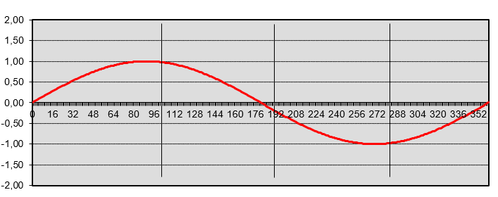
   • Sine values range between -1 and 1
   • Reaches maximum (1) at 90° (π/2 radians)

1. Periodicity: The sine function is periodic with 2π (360°) period

Important Notes:

• Excel requires angles in radians
• To convert degrees to radians:
  • Multiply by PI()/180, or
  • Use RADIANS() function
• The function returns results between -1 and 1

 Example:

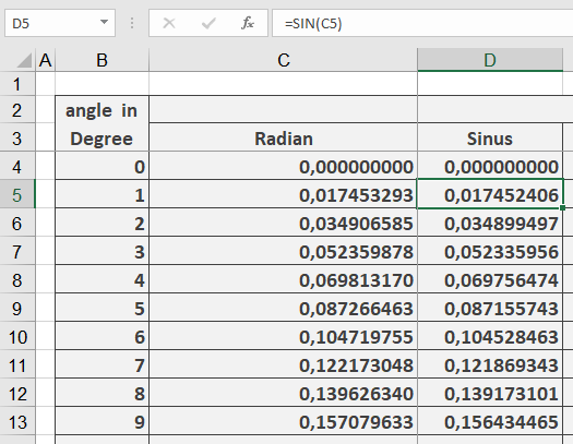
Visualization Tip:
The sine curve can be plotted with:

• x-axis: Angle (in radians)
• y-axis: SIN(x)
  This produces the characteristic wave pattern that oscillates between -1 and 1.

Common Applications:

1. Physics (wave motions)
2. Engineering (oscillations)
3. Navigation (distance calculations)
4. Computer graphics (wave patterns)

Its returns the sign of a number as:

• 1 if the number is positive
• 0 if the number is zero
• -1 if the number is negative

Syntax:
SIGN(number)

Argument:

Argument	Description
number (required)	Any real number.

Background:

• Positive numbers are > 0 (plus sign + optional).
• Negative numbers are < 0 (minus sign – required).
• Zero is neutral (neither positive nor negative).

Examples:

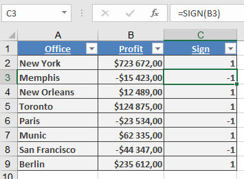
1. Filtering Negative Revenues

Scenario: Identify subsidiaries with losses in a sales list.

Step 1: Add a column with SIGN() to flag revenue signs:

=SIGN(B2)  // Returns -1 for losses, 1 for profits

Step 2: Calculate total losses (negative values):

{=SUM(IF(SIGN(B2:B9)=-1, B2:B9))}  // Array formula (Ctrl+Shift+Enter)

Step 3: Calculate total profits (positive values):

{=SUM(IF(SIGN(B2:B9)=1, B2:B9))}  // Array formula (Ctrl+Shift+Enter)

Additional Use Cases:

• Conditional Formatting: Highlight negative values.
• Data Validation: Restrict inputs to positive numbers.

Key Notes:

• Simple but powerful for data analysis and validation.
• Often combined with IF(), SUMIF(), or array formulas.

Its Calculates the sum of a power series with the formula:
y = a₁xⁿ + a₂xⁿ⁺ᵐ + a₃xⁿ⁺²ᵐ + … + aₖxⁿ⁺ᵏᵐ
The number of terms equals the number of coefficients provided.

Syntax:
SERIESSUM(x; n; m; coefficients)

Arguments:

Argument	Description
x (required)	Independent variable value for the series.
n (required)	Initial power of *x* (first term).
m (required)	Increment added to *n* for each subsequent term.
coefficients (required)	Array of coefficients (a₁, a₂, …, aₖ). Determines the number of terms.

Background:
A power series approximates functions using an expansion point (x₀). Accuracy improves with more terms:
Σ aₖ(x – x₀)ⁿ⁺ᵏᵐ

Examples:

Example 1: Calculating Euler’s Number (*e*)

Formula:

=SERIESSUM(1, 0, 1, {1, 1, 0.5, 0.16666667, 0.04166667, 0.00833333, 0.00019841})

Returns: 2.71686508

Coefficients Explained:

• a₁ = 1 = 1/0!
• a₂ = 1 = 1/1!
• a₃ = 0.5 = 1/2!
• …
• a₇ = 0.00019841 ≈ 1/6!

Example 2: Sine Function Approximation

1. Inputs (B3:C9):
   • *x* = π/4 (45° in radians)
   • Coefficients: {1, -0.166667, 0.008333, -0.000198} (Taylor series for sine)
2. Formula (Cell E7):

=SERIESSUM(B3, 1, 2, {1, -0.166667, 0.008333, -0.000198})

Result: 0.707107

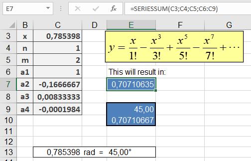
1. Validation:
   • =DEGREES(B3) → Confirms *x* = 45°
   • =SIN(B3) → Returns 0.707107 (matches SERIESSUM() to 6 decimals)

Key Notes:

• Used in engineering/math to approximate functions (e.g., eˣ, sin(x)).
• More coefficients → higher precision.
• Negative coefficients alternate signs (e.g., sine series).

This function rounds a number up (away from zero) to the specified number of digits.

Syntax:
ROUNDUP(number; num_digits)

Arguments:

• number (required) – The real number to be rounded up.
• num_digits (required) – The number of decimal places to round up to.

Key Behavior:
Unlike standard rounding (ROUND()), ROUNDUP() always rounds up regardless of the digit value.

Rules Based on num_digits:

• num_digits > 0: Rounds up to the specified decimal places.
• num_digits = 0: Rounds up to the nearest integer.
• num_digits < 0: Rounds up to the left of the decimal point (e.g., tens, hundreds).

Special Cases:

• Negative numbers round toward zero (e.g., -2.8 → -2).
• Zero or positive numbers round away from zero (e.g., 1.1 → 2).

Examples: