Votre panier est actuellement vide !
Catégorie : Excel function
How to use the ROUNDDOWN() function in Excel
This function rounds a number down (toward zero) to the specified number of digits.
Syntax:
ROUNDDOWN(number; num_digits)Arguments:
- number(required) – The real number to be rounded down.
- num_digits(required) – The number of decimal places to round down to.
Background:
Unlike ROUND(), which follows standard rounding rules (≥5 rounds up, <5 rounds down), ROUNDDOWN() always truncates the number at the specified digit, regardless of its value.Behavior based on num_digits:
- num_digits > 0: Rounds down to the specified decimal places.
- num_digits = 0: Rounds down to the nearest integer.
- num_digits < 0: Rounds down to the left of the decimal point (e.g., tens, hundreds).
Key Notes:
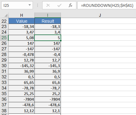
- Negative numbers are rounded toward zero(e.g., -2.846 → -2.84).
- The function simply truncates extra digits without rounding.
Examples:
How to use the ROUND() function in Excel
This function rounds a number to a specified number of decimal places.
Syntax:
ROUND(number; num_digits)Arguments:
- number (required) – The number you want to round.
- num_digits (required) – The number of decimal places to round to.
Background:
Rounding is essential in our number system, as most values are rounded at some point. Reasons for rounding include:- Improving clarity and simplifying calculations (e.g., demographic statistics, pi (π)).
- Standardizing monetary values (e.g., prices rounded to two decimal places, since the smallest unit is one cent).
Rounding Rules:
- If the digit after the rounding position is 5 or greater, the number is rounded up.
- If the digit is 4 or less, the number is rounded down.
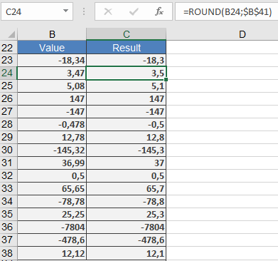
- Negative values are rounded away from zero (i.e., upward in absolute terms).
Examples:
- $3.2549 → $3.25 (4 ≤ 4, round down)
- $3.2551 → $3.26 (5 ≥ 5, round up)
- –$3.2549 → –$3.25
- –$3.2551 → –$3.26
Effect of num_digits:
- num_digits > 0: Rounds to the specified decimal places.
- num_digits = 0: Rounds to the nearest integer.
- num_digits < 0: Rounds to the left of the decimal point (e.g., tens, hundreds).
Example:
How to use the ROMAN() function in Excel
This function converts an Arabic numeral into a Roman numeral.
Syntax:
ROMAN(number ; form)Arguments:
- number (required) – The Arabic numeral to convert (must be between 0 and 3999). Negative numbers or values above 3999 return a #VALUE! error.
- form (optional) – A number specifying the Roman numeral style, ranging from Classic (0) to Simplified (4). Higher values produce more concise forms (see *Table 1*).
Table 1. Possible Values for the form Argument
Value Type of Roman Numeral 0 Classic 1 More concise 2 More concise 3 More concise 4 Simplified TRUE Classic FALSE Simplified Background:
Roman numerals consist of basic numerals and auxiliary numerals, the latter introduced to shorten lengthy representations (see *Table 2*).Table 2. Roman Numeral Forms
Basic Numeral Value Auxiliary Numeral Value I 1 V 5 X 10 L 50 C 100 D 500 M 1000 Rules for Roman Numerals:
- Addition: Identical adjacent numerals are added (max 3 in a row).
- Example: III = 3.
- Subtraction: A smaller numeral to the left of a larger one is subtracted; to the right, it is added. Auxiliary numerals (V, L, D) cannot be subtracted.
- Examples: XI = 11, IX = 9, XLV = 45.
- Subtraction Limits: Basic numerals (I, X, C) can only be subtracted from the nearest larger value.
- Examples: CD = 400, CM = 900.
Historically, Roman numerals were used in Europe until the 16th century, with adjustments over time. The subtractive notation (e.g., IV for 4) was not originally used—clocks often display 4 as IIII.
Examples:
The ROMAN() function is useful for chapters, lists, or enumerations: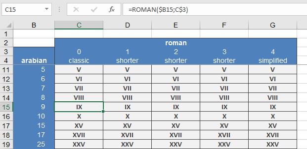
How to use the RANDBETWEEN() function in Excel
This function returns a random integer from a specified range. A new random number is generated every time the worksheet is recalculated.
Syntax:
RANDBETWEEN(bottom; top)Arguments:
- bottom(required) – The smallest integer RANDBETWEEN() can return.
- top(required) – The largest integer RANDBETWEEN() can return.
Background:
Random values are essential in engineering and natural sciences for simulating processes.
To generate a random date, the input must be provided as a numerical value.Example:
the practical example for the RANDBETWEEN() function.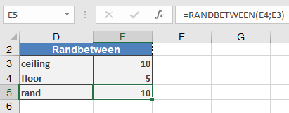
How to use the RAND() function in Excel
This function returns a random number between 0 and 1 with up to 16 decimal places.
Syntax:
RAND()Arguments:
NoneBackground:
The RAND() function returns a random number greater than or equal to 0 and less than 1.To generate a random real number between a and b, use:
=RAND() • (b – a) + aA new random number is returned every time the worksheet is calculated.
Example:
The RAND() function is often used to fill a table with test data or to simulate processes in engineering and natural sciences. The formula must be entered in each cell. Some examples of this function are: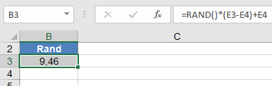
How to use the RADIANS() Function in Excel
Its converts an angle from degrees to radians.
Syntax
RADIANS(angle)
Argument
Parameter Requirement Valid Input angle Required Angle in degrees (°) Key Properties
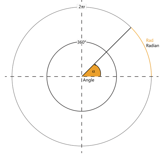
- Conversion Formula:
radians=degrees×(π180)
-
- π in Excel: PI() ≈ 3.14159265358979.
- Critical Values:
Degrees Radians 0° 0 30° π/6 ≈ 0.5236 45° π/4 ≈ 0.7854 90° π/2 ≈ 1.5708 180° π ≈ 3.1416 360° 2π ≈ 6.2832 - Inverse Function:
- DEGREES() converts radians back to degrees.
Examples
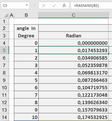
- Basic Conversion:
=RADIANS(1) → Returns 0.017453293
=RADIANS(45) → Returns 0.785398163
=RADIANS(90) → Returns 1.570796327
- Trigonometric Calculations:
=SIN(RADIANS(30)) → Returns 0.5 (sin of 30°)
- Real-World Use:
- Navigation: Convert nautical miles to radians for arc length.
- Physics: Angular velocity calculations.
Why This Matters
- Excel’s Default: Trigonometric functions (SIN, COS, TAN) use radians.
- Precision: Avoids manual conversion errors.
- Scientific Standards: Radians are natural units in calculus/physics.
Related Functions
- DEGREES(): Radians to degrees.
- SIN()/COS()/TAN(): Trigonometric functions.
- PI(): Returns π for manual calculations.
How to use the QUOTIENT() Function in Excel
Its returns the integer portion of a division operation (without the remainder).
Syntax
QUOTIENT(numerator; denominator)
Arguments
Parameter Requirement Valid Input numerator Required Dividend (number to divide) denominator Required Divisor (must be ≠ 0) Key Properties
- Behavior:
- Truncates (not rounds) the result toward zero.
- Equivalent to INT(numerator/denominator) for positive numbers.
- Ignores remainder: QUOTIENT(5, 2) = 2 (remainder 1 is dropped).
- Error Handling:
- #DIV/0! if denominator = 0.
- #VALUE! for non-numeric inputs.
- Mathematical Equivalent:

Examples
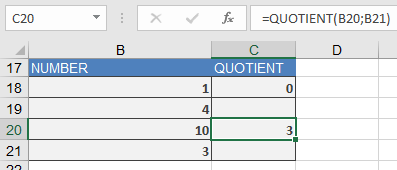
- Paint Mixing Example:
=QUOTIENT(1, 4) → Returns 0 (since 1/4 = 0.25, integer part is 0)
- Real-World Use:
- Inventory: Full crates from total items (=QUOTIENT(total_items, items_per_crate)).
- Timekeeping: Complete hours worked (=QUOTIENT(minutes, 60)).
Comparison with Similar Functions
Function Example (10, 3) Notes QUOTIENT() 3 Drops remainder / 3.333… Full decimal result INT(numerator/denominator) 3 Same as QUOTIENT for positives TRUNC(numerator/denominator) 3 Identical to QUOTIENT Why This Matters
- Efficiency: Faster than INT() or TRUNC() for integer division.
- Clarity: Explicitly signals intent to discard remainders.
- Compatibility: Requires Analysis ToolPak in older Excel versions.
Related Functions
- MOD(): Returns the remainder.
- INT()/TRUNC(): Alternative truncation methods.
- ROUND(): Controlled rounding.
- Behavior:
How to use the PRODUCT() Function in Excel
This function multiplies all given numbers or ranges and returns the product.
Syntax
PRODUCT(number1; [number2]; …)
Arguments
Parameter Requirement Valid Input number1 Required Number, cell reference, or range number2,… Optional Additional numbers/ranges (up to 255 total) Key Properties
- Behavior:
- Multiplies all numeric values in arguments.
- Ignores empty cells, text, or logical values (TRUE/FALSE).
- Returns 0 if any argument is zero.
- Mathematical Notation:
PRODUCT(a,b,c)=a×b×c
-
- Analogous to the Π (Pi) symbol in mathematics for sequential products.
- Alternatives:
- Use the * operator for simple multiplication: =A1*A2*A3.
Examples
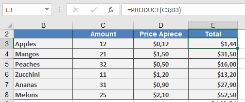
Why This Matters
- Efficiency: Faster than manual * chains for large ranges.
- Error-Resistant: Skips non-numeric values automatically.
- Financial/Statistical Use:
- Compound growth calculations.
- Volume/area computations.
Related Functions
- SUMPRODUCT(): Multiplies then sums ranges.
- SUM(): Adds values.
- FACT(): Factorial (product of integers up to *n*).
- Behavior:
How to use the POWER() Function in Excel
Its returns the result of raising a base number to a specified exponent.
Syntax
POWER(number; power)
Arguments
Parameter Requirement Valid Input number Required Any real number (base) power Required Real number (exponent) Key Properties
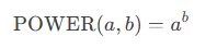
- Mathematical Operation:
-
- Special Cases:
- a0=1 (any non-zero aa)
- 0b=0 (for b>0b>0)
- a1=a
- Special Cases:
- Error Handling:
- #NUM! if a<0a<0 and bb is non-integer (e.g., (−2)1.5(−2)1.5).
- Alternate Syntax:
Use the caret operator (^):
=5^2 // Equivalent to =POWER(5,2)
Examples
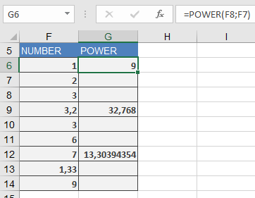
- Basic Calculations:
=POWER(3, 2) → Returns 9
=POWER(3.2, 3) → Returns 32.768
=POWER(7, 1.33) → Returns ≈13.3039
- Computer Science (Binary Units):
=POWER(2, 10) → Returns 1024 (1 kilobyte)
- Physics (Inverse Square Law):
=POWER(distance, -2) → Calculates intensity decay.
Related Functions
- SQRT(): Square root (=POWER(x,0.5)).
- EXP(): Natural exponentiation (exex).
- LOG(): Inverse of power functions.
How to use the ODD() Function in Excel
Its rounds a number away from zero to the nearest odd integer.
Syntax
ODD(number)
Argument
Parameter Requirement Valid Input number Required Any real number Key Behavior
- Rounding Rules:
- Positive numbers: Rounds up to next odd integer.
- =ODD(1.9) → 3 (next odd above 1.9)
- Negative numbers: Rounds down to next odd integer (more negative).
- =ODD(-2.8) → -3 (next odd below -2.8)
- Odd integers: Returns unchanged.
- =ODD(5) → 5
- Positive numbers: Rounds up to next odd integer.
- Error Handling:
- #VALUE! for non-numeric inputs.
- Special Cases:
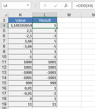
Input Output Explanation 0 1 Rounds away from zero -1 -1 Already odd 2.1 3 Next odd above Examples
Comparison with Similar Functions
Function Direction Target Example (Input: 2.5) ODD() Away from zero Next odd 3 EVEN() Away from zero Next even 4 CEILING() Up Specified multiple Depends on significance FLOOR() Down Specified multiple Depends on significance Why This Matters
- Data Standardization: Enforce odd-numbered IDs or codes.
- Mathematical Modeling: Odd-step simulations (e.g., cellular automata).
Related Functions
- EVEN(): Rounds to nearest even integer.
- INT(): Truncates to integer (toward zero).
- MROUND(): Rounds to specified multiple.
- Rounding Rules: