Votre panier est actuellement vide !
Catégorie : Excel VBA Course
Applying Styles to Excel Tables
Once you’ve created a table in Excel, the first thing you’ll likely want to do is make it visually appealing and easy to interpret. Thankfully, Microsoft Excel offers a wide array of built-in table styles that allow you to instantly format or reformat a table with just one click. And if none of the default styles meet your specific design preferences, you can quickly define your own custom style.
Moreover, Excel allows you to toggle key table elements on or off — such as the header row, banded rows, total row, and more — giving you full control over the appearance and behavior of your table.
Built-in Table Styles
Excel tables are designed not just for data storage but for enhanced data management. They offer features like built-in filtering and sorting, calculated columns, structured references, and automatic total rows. When you convert a regular data range into a table, Excel automatically applies default formatting: alternating row colors (banded rows), border lines, and font styling.
If you’re not satisfied with the default format, you can easily change it via the Design tab that appears under Table Tools when a cell in the table is selected.
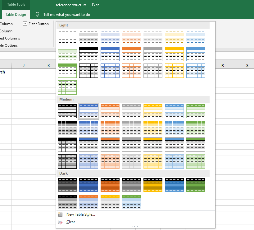
Example: Over 50 Built-in Table Styles
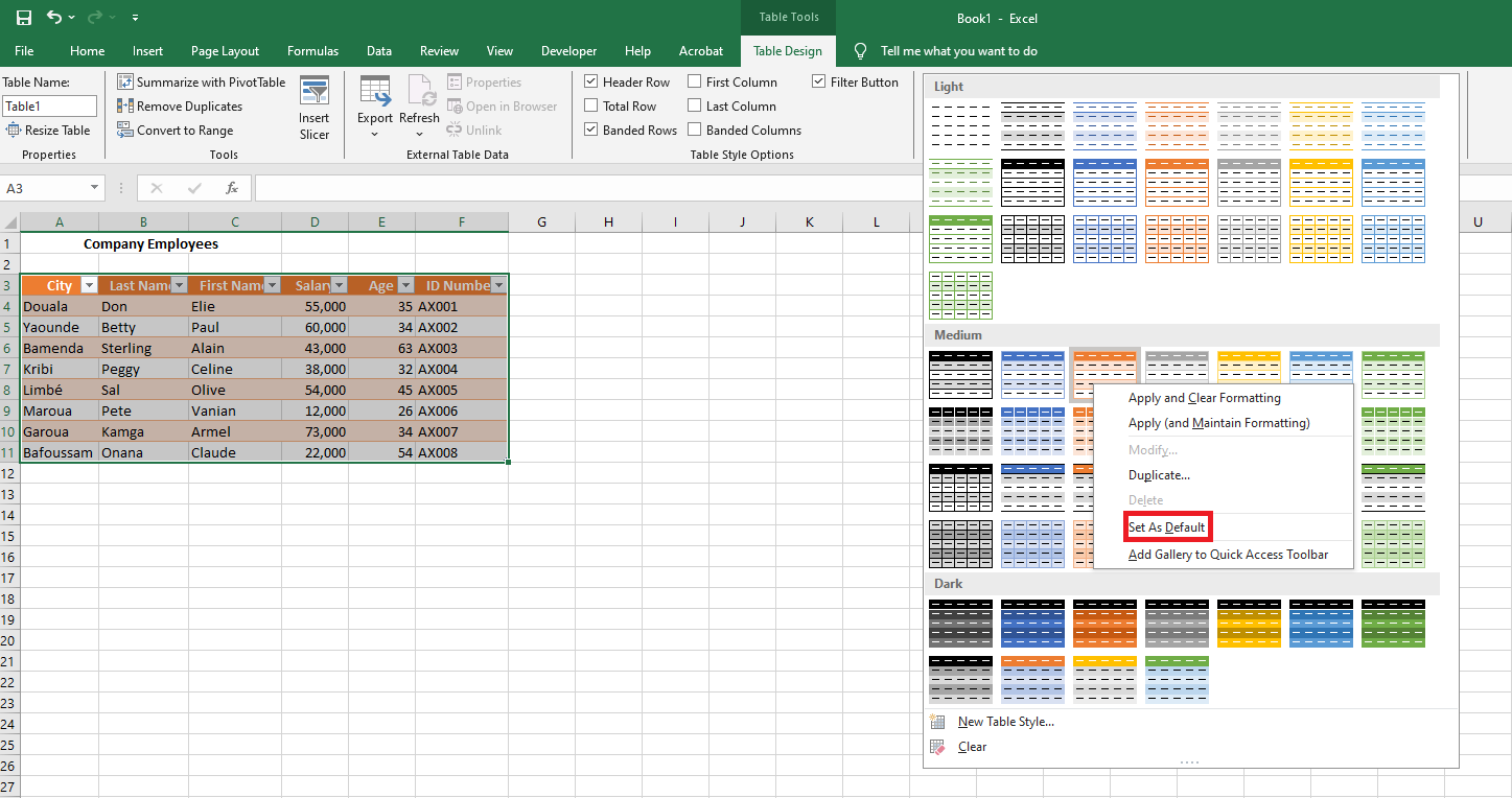
As shown in the illustration (Fig. 3.2.1.a), Excel provides a gallery of over 50 pre-defined styles, categorized as Light, Medium, and Dark themes. A table style acts as a formatting template, automatically applying visual elements to headers, rows, columns, and the total row.
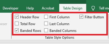
You can further customize your table using the Table Style Options, which allow you to control the appearance of specific elements:
-
Header Row – Show or hide the table headers.
-
Total Row – Add a summary row at the bottom of the table, with built-in functions for each column.
-
Banded Rows / Columns – Alternate shading for improved readability.
-
First/Last Column – Apply special formatting to highlight these columns.
-
Filter Button – Show or hide the dropdown filter arrows in the header row.
Choosing a Table Style While Creating a Table
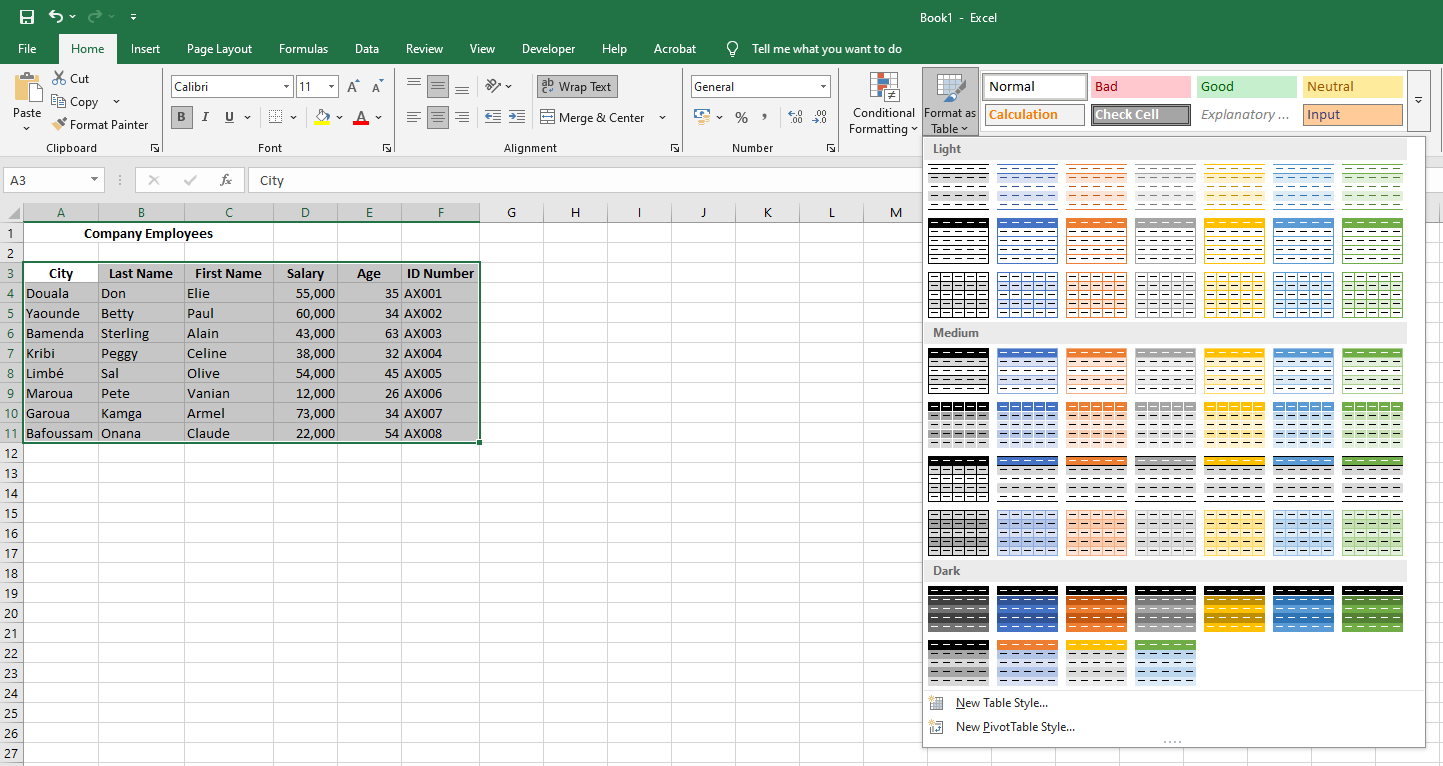
To create a table and immediately apply a specific style, follow these steps:
-
Select the cell range you want to convert into a table.
-
On the Home tab, go to the Styles group, and click Format as Table.
-
In the style gallery, click the table style you want to use.
Changing the Style of an Existing Table
To change the appearance of a table that already exists:
-
Click any cell inside the table.
-
Go to the Design tab under Table Tools, and in the Table Styles group, click the More arrow to see all available styles.
-
Hover over a style to preview it live on your table. Click to apply it.
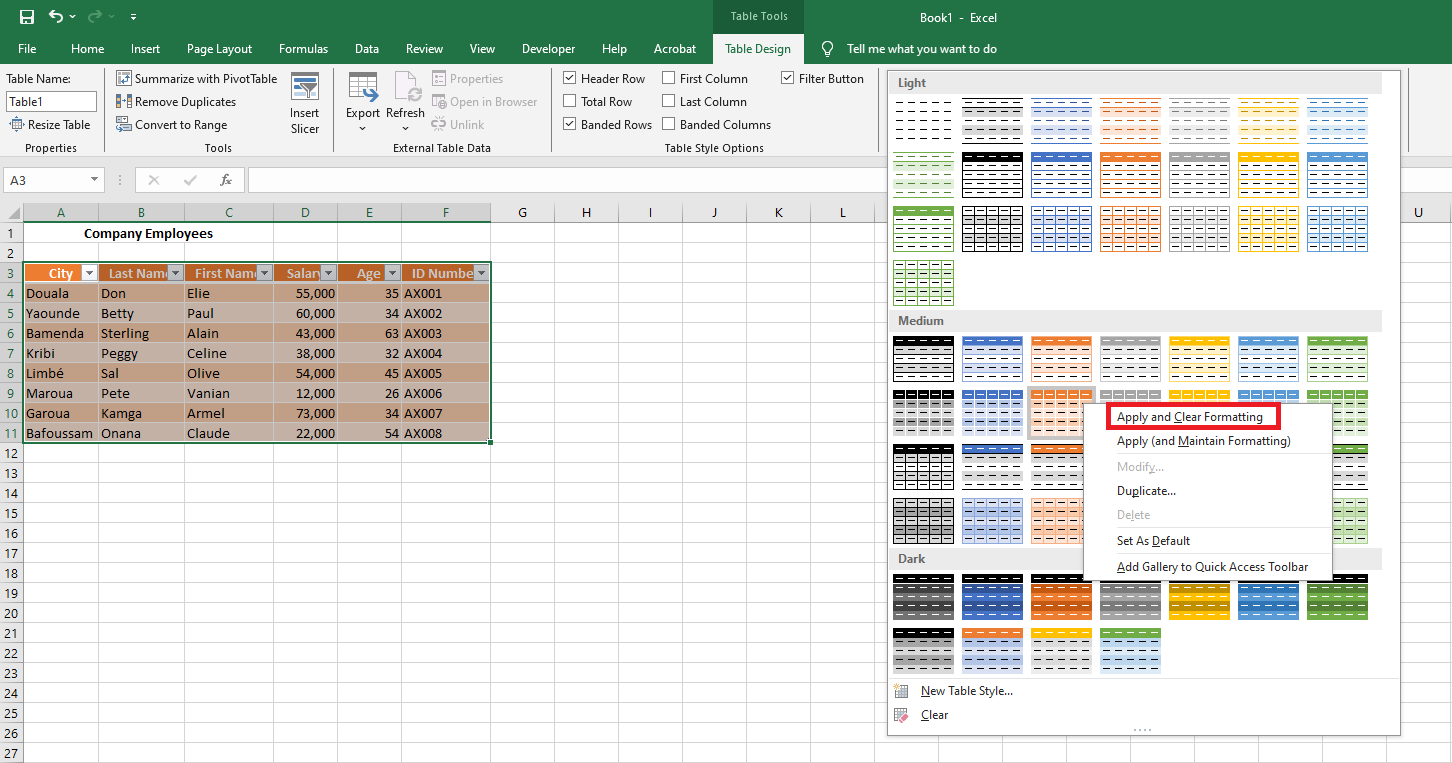
Tip: If you previously applied custom formatting (like bold fonts or custom colors) manually to some cells, Excel will retain them even when you switch styles. To override this and apply the new style completely, right-click the style and choose Apply and Clear Formatting.
5.4 Setting a Default Table Style for a Workbook
If you want every new table in your workbook to follow a specific style, set it as the default:
-
In the Table Styles gallery, right-click your preferred style.
-
Select Set As Default.
From now on, every table inserted via the Insert tab will adopt this style automatically.
Applying Table Styles Without Creating an Actual Table
If your goal is to quickly style a data range without converting it into a structured Excel table, here’s a workaround:
-
Select the data range you wish to format.
-
On the Home tab, in the Styles group, click Format as Table, then choose your desired style.
-
After the table is created, go to the Design tab and click Convert to Range to revert it back to a regular range.
-
Structured References in Excel Tables
One of the most powerful and practical features of Excel tables is the use of structured references. At first glance, this special syntax for referencing table data may appear complex or even confusing, especially if you’re accustomed to traditional cell references. However, once you begin to work with it, you’ll quickly discover how useful and efficient this functionality can be—especially in dynamic data environments.
A structured reference, also known as a table reference, is a specific way to refer to parts of an Excel table by using the table’s name and column headers, rather than standard cell addresses like A1 or B2. This makes formulas easier to read, more intuitive, and more resilient to changes.
The reason this type of referencing is so essential lies in the inherent power of Excel tables: unlike regular cell ranges, tables automatically expand or contract when data is added or removed. Standard cell references do not adapt to these changes, which can lead to inaccurate results or broken formulas. Structured references, on the other hand, dynamically adjust to include new rows or columns, ensuring that your formulas always remain up to date.
For instance, to sum the values from cells B2 to B5 using a regular cell range, you would write:
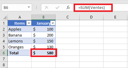
=SUM(B2:B5)But if your data is organized in an Excel table named SalesTable, and you want to sum the values in the « Sales » column, you would use a structured reference like this:
=SUM(SalesTable[Sales])This formula is not only easier to interpret (you know exactly what it sums), but it will also automatically include any new sales data added to the table.
Key Features of Structured References in Excel
Compared to standard cell references, structured references offer several advanced features that enhance both the flexibility and efficiency of working with data in Excel tables:
■ Easy to Create
Structured references are incredibly simple to insert into a formula. You don’t need to memorize any special syntax—just select the desired table cells with your mouse, and Excel automatically generates the correct structured reference. This makes it accessible even to users unfamiliar with the syntax.■ Automatically Resilient and Self-Updating
One of the greatest advantages of structured references is their ability to automatically adapt to changes. When you rename a column in a table, all associated structured references are immediately updated to reflect the new column name—eliminating the risk of broken formulas. Furthermore, when you add new rows to the table, those rows are seamlessly included in existing references, ensuring that formulas always cover the entire data range.This means that no matter how frequently your data changes, your structured references remain accurate and up to date, reducing the need for manual adjustments.
■ Usable Both Inside and Outside the Table
Structured references are not limited to formulas within the table itself. You can also use them in formulas located outside the table, which is especially helpful in large workbooks where you may need to reference specific tables from various sheets. This improves clarity and makes it easier to manage complex spreadsheets.■ Auto-Fill for Calculated Columns
When you enter a formula in a single cell of a table column, Excel automatically fills the rest of the column with the same formula—creating what’s known as a calculated column. This feature ensures consistency in your computations and saves time by applying the formula to all rows without manual copying.How to Create a Structured Reference in Excel
Creating a structured reference in Excel is both straightforward and intuitive. If you’re starting with a regular range of data, your first step should be to convert that range into an official Excel table. This unlocks all the advanced features of table management, including structured references.
To convert a standard data range into a table:
-
Select the entire dataset.
-
Press Ctrl + T (or Ctrl + L in some older versions of Excel).
-
Make sure the « My table has headers » option is checked, then click OK.
Once your data is formatted as an Excel table, you can create structured references by following these simple steps:
- Begin writing your formula
Start as usual by typing the equals sign (=) in the desired cell. - Select the relevant cells in the table
Instead of typing cell addresses, simply use your mouse to select the cell or range you want to include from within the table. Excel will automatically insert the structured reference using the table name and column headers. This eliminates the need to know the syntax by heart. - Close the formula and press Enter
Once your structured reference is inserted, complete the formula by typing the closing parenthesis)and pressing Enter. If you’re entering the formula inside the table, Excel will automatically fill the entire column with the same formula, creating a calculated column.
Example: Summing Monthly Sales
Suppose you have a table namedMonthlySales, and it contains sales figures for three months across columns B, C, and D. You want to calculate the total sales per row in column E.To do this:
-
Click in cell E2 (the first row of your total column).
-
Type:
=SUM( -
Select the cells B2 to D2 (Excel will translate this into a structured reference like =SUM(Article[@[January]:[March]]) depending on your column headers).
-
Type the closing parenthesis
)and press Enter.
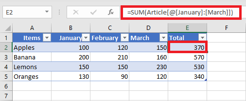
As a result, the entire column E is automatically filled with the following formula:
=SUM(MonthlySales[@[January]:[March]])Even though the formula looks identical across all rows, Excel evaluates it individually for each row using the respective data. This row-wise behavior is one of the most powerful aspects of structured references in Excel tables.
Creating Structured References Outside of a Table
If you’re entering a formula outside of the table and only need to refer to a specific column or range of data within the table, you can quickly create a structured reference without manually selecting the cells. Here’s how:
- Begin typing the formula normally.
For example, to calculate the maximum value in a column, you might start typing=MAX(. - Type the first few letters of the table name.
As soon as you type the first letter, Excel will display a dropdown list of all table names that match what you’re typing. The more letters you type, the more refined the list becomes. - Use the arrow keys to select the correct table.
Scroll through the list using the up/down arrow keys on your keyboard. - Press Tab or double-click to insert the table name.
Once the correct table is selected, press Tab or double-click the name to insert it into your formula. - Complete the formula and press Enter.
Add any column reference or closing parentheses needed and press Enter.
Example:
Let’s say you want to find the highest value in a table named Article.-
You begin by typing
=MAX( -
Then type “Ar”
-
Excel shows Article as a suggestion
-
Press Tab to select it
-
Complete the formula with
)and hit Enter
Your final formula looks like this:
=MAX(Article)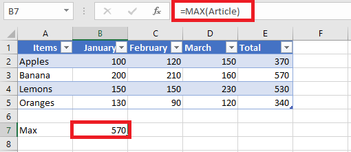
Structured Reference Syntax in Excel
As previously mentioned, you don’t necessarily need to master the syntax of structured references to use them in formulas—Excel inserts them automatically as you work with tables. However, understanding this syntax will help you interpret what your formulas are actually doing, especially when analyzing or debugging them.
In general, a structured reference is a text string that starts with the table name and ends with one or more column specifiers. To illustrate, let’s break down the following formula which adds the values from the “South” and “North” columns in a table named Regions:
This structured reference contains three main components:
-
Table name
-
Item specifier
-
Column specifier(s)
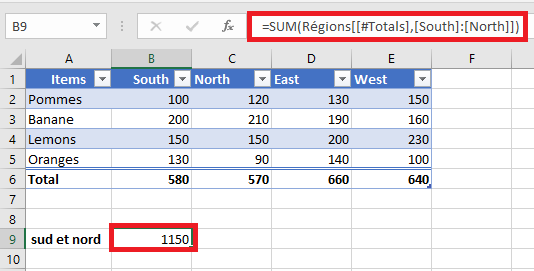
When you select the cell containing this formula and click into the formula bar, Excel highlights the exact cells involved in the calculation, helping you visualize the data being referenced.
Table Name
The table name refers only to the data body of the table—it excludes both the header row and the total row. This name may be the default (e.g.,
Table1) or a custom name likeRegions.
If your formula is located inside the same table, Excel often omits the table name because it is implicitly understood.Column Specifier
A column specifier refers to the data within a specific column, excluding the header and total rows. It is written inside square brackets.
For example:To reference multiple adjacent columns, you can use a range operator (colon), like this:
If a column name contains spaces, punctuation, or special characters, Excel adds an extra set of square brackets:
Item Specifier
To reference specific parts of a table (such as the entire table or just the headers), Excel uses item specifiers. These always begin with a hash symbol (
#) except for row-specific references using@.Item Specifier Description [#All]Refers to the entire table (data, headers, and totals) [#Data]Refers only to the data rows [#Headers]Refers to the column headers [#Totals]Refers to the total row (returns null if the total row is not visible) [@ColumnName]Refers to the same row as the formula, within the specified column For example, to sum values from the South and West columns in the current row, you would write:Structured Reference Operators
Structured references support various operators that enhance their flexibility:
• Range Operator (
:)Used to reference a range of adjacent columns. For example:
This sums the current row’s values from “South” to “West”.
• Union Operator (
,comma)Used to reference non-adjacent columns. For instance:
This adds values from the “South” and “West” columns in the same row.
• Intersection Operator (
Used to refer to the value at the intersection of a specific row and column. For example, to return the value at the intersection of the Total row and the West column:
Note: In this case, the
[#All]specifier (or a similar item specifier) is essential, because column specifiers alone do not include the total row. Without it, Excel may return a#NULL!error.Syntax Rules for Structured Table References
When manually editing or creating structured references in Excel tables, it’s important to follow specific syntax rules to ensure formulas work properly and remain readable. Below are the main guidelines to follow:
Enclose Specifiers in Brackets
All column specifiers and special item identifiers must be enclosed in square brackets[ ]. If a specifier includes multiple elements or a range, it should be wrapped in an additional set of brackets.
Example:
To reference a range from the “South” column to the “West” column in the current row:=Regions[@[South]:[West]]Separate Multiple Specifiers with Commas or Semicolons
When combining two or more inner specifiers within a single reference, separate them with commas (,in English versions) or semicolons (;in French versions), depending on your regional Excel settings.
Example:
To reference the column header for « South » within a structured reference, use an additional set of brackets and separate specifiers:=Regions[[#Headers],[South]]Do Not Use Quotation Marks Around Column Headers
In structured references, column headers should not be enclosed in double quotes—even if they contain text, numbers, or dates. Excel automatically interprets them based on the table’s metadata.Use Single Quotes for Special Characters in Column Headers
Certain characters within column headers—such as square brackets[ ], the pound/hash symbol#, and the single quote'—have special meaning in Excel. If one of these appears in a column name, precede it with a single quote (') within the reference to avoid syntax errors.
Example:
If a column is namedItem #, you must escape the#with a single quote:=Regions[[#Headers],[Item '#]]Use Spaces to Improve Readability
While not mandatory, inserting spaces between specifiers (especially after commas or semicolons) improves the clarity and readability of complex structured references.
Example:
To average the values in columns “South”, “North”, and “West” from the current row, you can use:=AVERAGE(Regions[@[South]]; Regions[@[North]]; Regions[@[West]])Structured References in Excel Tables
To better understand how structured references work in Excel tables, let’s review a few practical and illustrative examples. These examples are designed to be simple, meaningful, and applicable to real-world scenarios.
Counting Rows and Columns in an Excel Table
To determine the number of columns or rows in a table, you can use the built-in Excel functions
COLUMNSandROWS, which only require the table name as input:These formulas return the total number of columns and data rows in the table named
Sales.If you want to include both the header row and the Total Row (if present), use the special item specifier
[#All]:=ROWS(Sales[#All])This will return the number of all rows including the header and total rows.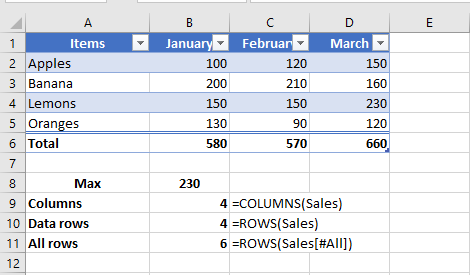
Counting Blank and Non-Blank Cells in a Specific Column
When working with a specific column in a table, you may want to count how many cells are empty or contain data. Be sure to place your formula outside of the table to avoid circular references and incorrect results.
-
To count blank cells:
-
To count non-blank cells:
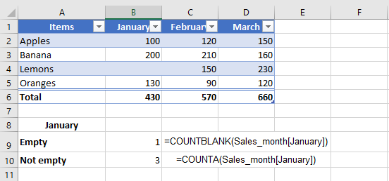
If your table is filtered and you want to count only the non-blank cells in the visible rows, use the
SUBTOTALfunction with function number103:This version of the formula ignores filtered-out (hidden) rows and only counts visible non-empty cells.
Summing Values in an Excel Table
The fastest way to calculate totals in an Excel table is by enabling the Total Row option:
-
Right-click anywhere inside the table.
-
Select Table from the context menu.
-
Click Total Row.
Excel will add a summary row at the bottom of the table. By default, it may only calculate the total for the last column, leaving the rest empty.
To fix this, click any empty cell in the Total Row, click the dropdown arrow that appears, and choose the SUM function. Excel will insert a structured
SUBTOTALformula that adds only the values from visible rows, ignoring any filtered-out data:Likewise, a regular
SUMfunction using a structured reference (e.g.,=SUM(Sales[January])) won’t work inside the table for the same reason.Relative and Absolute Structured References in Excel
By default, structured references in Excel tables behave according to specific rules, which can impact how formulas respond when copied or dragged across cells:
-
References to multiple columns are absolute by nature. They do not change when the formula is copied or moved across the worksheet.
-
References to a single column are relative when formulas are dragged horizontally across columns, meaning the column reference will adjust. However, when such formulas are copied and pasted using standard commands (Ctrl+C and Ctrl+V), the references remain fixed.
This behavior presents a challenge when you need a combination of relative and absolute references in your table formulas. Dragging a formula will shift single-column references (which may be undesired), while copying and pasting will fix all references (removing the intended dynamic behavior). Fortunately, there are practical tricks to control this behavior precisely.
Absolute Structured Reference to a Single Column
To force a single-column reference to behave like an absolute reference, repeat the column name to explicitly define it as a range.
-
Relative column reference (default):
TableName[Column] -
Absolute column reference:
TableName[[Column]:[Column]]
To refer to the current row with an absolute column reference, use the
@symbol before the column name:-
TableName[@[Column]:[Column]]
Example Use Case
Imagine you want to sum the monthly sales of a specific product over three months. You enter the product name in cell
F2, and use theSUMIFfunction to calculate the total sales for January:However, if you drag this formula to the right to calculate totals for February and March, the
[Items]reference might shift, breaking the formula.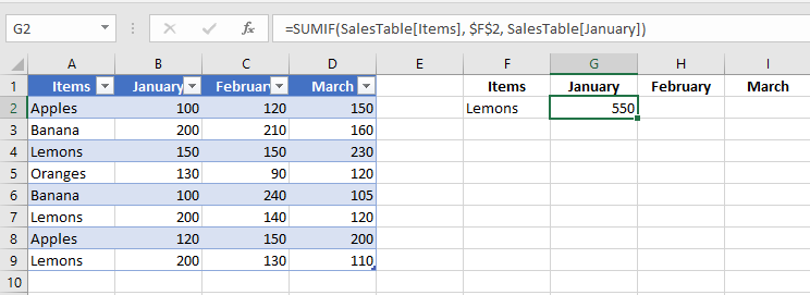
To prevent this, make the
[Items]reference absolute while keeping[January]relative:=SUMIF(SalesTable[[Items]:[Items]], $F$2, SalesTable[January])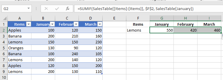 Now, when you drag the formula to adjacent columns, only the third argument (
SalesTable[January]) updates accordingly (to February, March, etc.), while the[Items]column remains fixed.Relative Structured References to Multiple Columns
By default, multi-column structured references in Excel tables are absolute and do not change when copied across cells. This default behavior is generally consistent and expected.
However, if you want to create a relative multi-column structured reference, you can do so by prefixing each column with the table name and removing the outer brackets.
-
Absolute range reference (default):
TableName[[Column1]:[Column2]] -
Relative range reference:
TableName[Column1]:TableName[Column2]
To reference multiple columns in the current row, use the
@symbol with each column:-
@[Column1]:[Column2]
Example: Row-Level Summation
To sum the values in the current row for columns January and February, use:
This reference is absolute, so copying it to another column will still sum January and February.
If you want the referenced columns to adjust relative to the formula’s position, use a relative structured reference like this:
=SUM(Table10[@February]:Table10[@March])
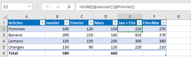
Note that if the formula is written inside the same table, the table name (
Table10) is optional and usually omitted by Excel automatically.-
Difference Between a Data List and an Excel Table
A data list in Excel is simply a range of related information organized in rows and columns. However, when that list is formally converted into an Excel Table, it gains powerful built-in features that enhance data management, analysis, and formatting. Below is a detailed comparison highlighting the key differences between a basic data list and an Excel Table:
Feature Data List Excel Table Header Row Headers must be added manually above the data. You can use multiple rows, and the headers don’t need to be unique. Excel automatically creates a single, dedicated header row. Each column header must be unique. You can easily toggle the visibility of the header row via the ribbon. Data Rows Rows are inserted or deleted manually by selecting ranges. Excel does not restrict these actions, which can lead to formatting errors or broken formulas. Rows are managed using table-aware commands. Excel ensures structural integrity by applying changes to entire rows and maintaining consistent formatting and formulas. Total Row Totals must be added manually beneath the list, and formulas for aggregation (SUM, AVERAGE, etc.) must be entered manually. Excel provides an optional Total Row that can be toggled on or off from the ribbon. Aggregation functions are easily applied using dropdown menus in each column. Sorting and Filtering Sorting and filtering are available, but Excel may prompt you to expand your selection if it doesn’t recognize the data range as structured. Sorting and filtering are built into the table structure. Excel inherently understands the table boundaries, eliminating the need to confirm data ranges. Formatting Formatting must be applied manually. When new rows are added, formatting may not automatically carry over. Excel automatically applies consistent formatting, including banded rows and table styles. New data entries inherit the table’s style by default. Formulas Standard cell references (e.g., A2:A10) must be used and managed manually. Copying or editing formulas across rows may introduce inconsistencies. Tables use structured references (e.g., =SUM(Table1[Sales])), which are more intuitive and robust. Excel automatically applies and updates formulas across all relevant rows.Conclusion
Using an Excel Table instead of a simple data list brings numerous benefits, including improved data integrity, easier formatting, automated calculations, and enhanced readability. Tables are especially helpful when working with dynamic datasets, allowing users to focus more on insights and less on manual adjustments.Resizing an Excel Table
Excel tables are dynamic and can easily be resized to include more or fewer rows and columns, depending on the evolving needs of your data. There are three main ways to resize a table:
-
Adding or removing rows and columns
-
Using the « Resize Table » command
-
Dragging the table corner to adjust its range
Adding or Removing Rows and Columns
Even after a table has been created, you can expand or reduce its size by adding or deleting rows or columns. Whether you insert data directly adjacent to the table or within its current range, Excel automatically applies the table’s formatting style.
To quickly insert a row or column adjacent to a table:
-
Click in a blank cell next to the table’s current boundary.
-
Enter a value into that cell.
-
Press Enter or click elsewhere to confirm. Excel will automatically include the new cell within the table range and apply the existing formatting.
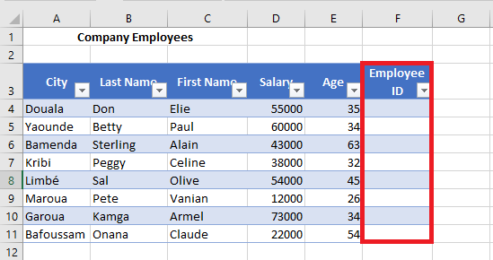
Note: When you type a formula into an empty column of a table, Excel automatically propagates that formula throughout the column — even for newly inserted rows — without needing to use AutoFill manually.
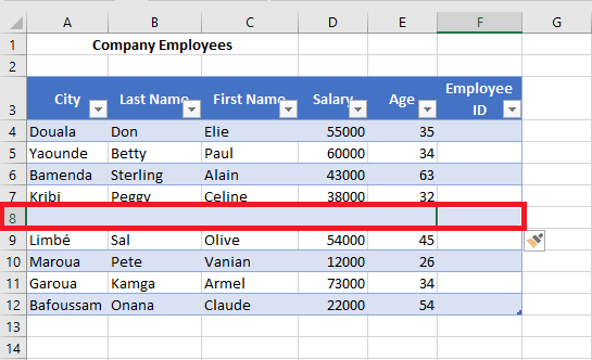
To insert a row or column using the Ribbon:
-
Select any cell within the table, directly next to where you want to add the new row or column.
Note: You cannot select a column header to use these insertion options. -
Go to the Home tab, click on the Insert drop-down arrow.
-
Choose one of the following options:
-
Insert Table Rows Above – adds a new row above the selected row.
-
Insert Table Columns to the Left – adds a new column to the left of the selected column.
-

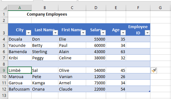
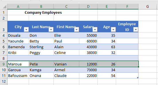
To delete unwanted rows or columns from a table:
-
Select a cell within the row or column you want to remove.
-
Click the Delete drop-down from the Ribbon.
-
Choose:
-
Delete Table Rows
-
Delete Table Columns
-
Resizing a Table Using the « Resize Table » Command
The Resize Table command allows you to explicitly define a new data range for the table. This method is especially useful when you want precise control over the dimensions of the table.
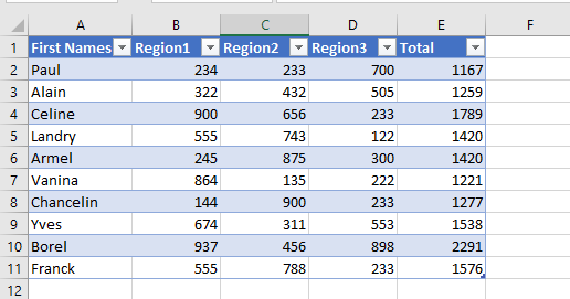
Steps:
-
Click on any cell inside the table.
-
Go to the Table Design tab (visible only when a table cell is selected).
-
Click on Resize Table.
-
In the input field that appears, type the new range you want for the table (e.g.,
A1:E14).

-
Click OK.
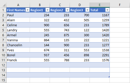
The table will be resized accordingly, either expanding or contracting to fit the specified range.
Resizing a Table by Dragging Its Corner
You can also manually resize a table by using the resize handle — a small icon located at the bottom-right corner of the table.
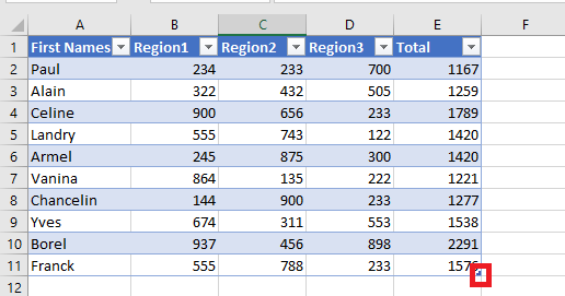
To reduce the table size:
-
Hover over the bottom-right corner of the table until the resize handle appears.
-
Click and drag inward to the desired range, e.g., from
A1:E11toA1:B11.
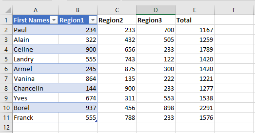
Note: Cells outside the new table range are no longer part of the table structure, lose their formatting, and no longer participate in formulas referencing the table.
To expand the table size:
-
Hover over the bottom-right corner and click the resize handle.
-
Drag outward to include more rows and/or columns, e.g., from
A1:B11toA1:G11.

The newly added cells are automatically formatted to match the existing table style, and the table’s internal links and formulas extend to include them.
-
Working with Excel Tables and Ranges
Excel tables are among the most powerful features for managing, calculating, and updating structured datasets efficiently. While tables provide enhanced functionality like automatic expansion, structured references, and built-in filters, there may be cases where you need to revert a table back to a regular range—or convert a standard range into a fully functional table.
How to Convert an Excel Table to a Normal Range
If you wish to remove table functionality while keeping your data intact, Excel offers a quick way to convert a table into a normal range. Follow these steps:
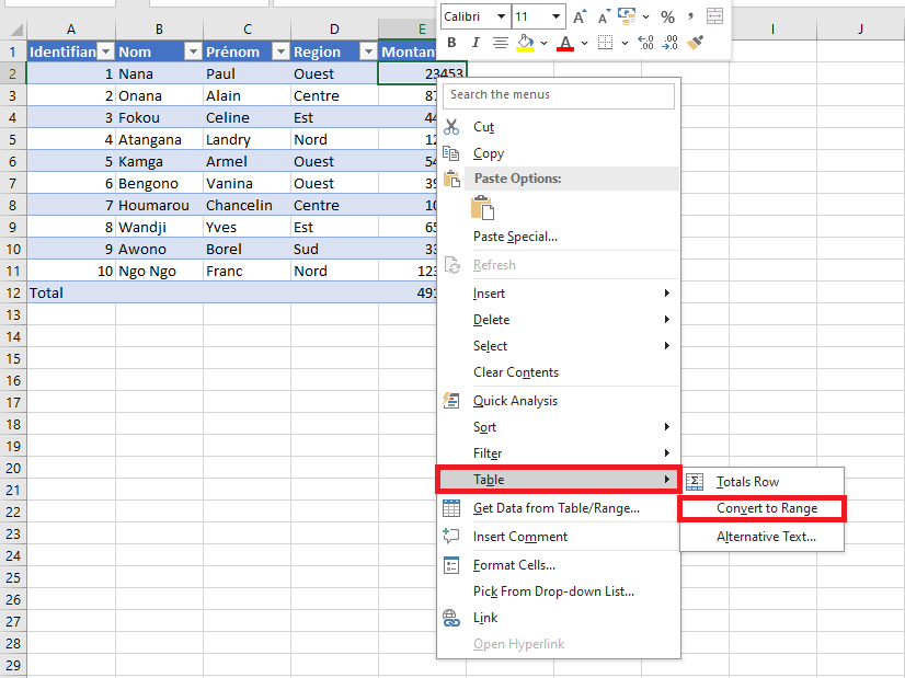
- Method 1 (Right-click method):
Right-click any cell within the table. From the context menu, select Table > Convert to Range.
- Method 2 (Using the Ribbon):
- Select any cell in the table to activate the Table Design tab.
- On the Table Design tab (formerly « Design » in older versions), locate the Tools group and click Convert to Range.
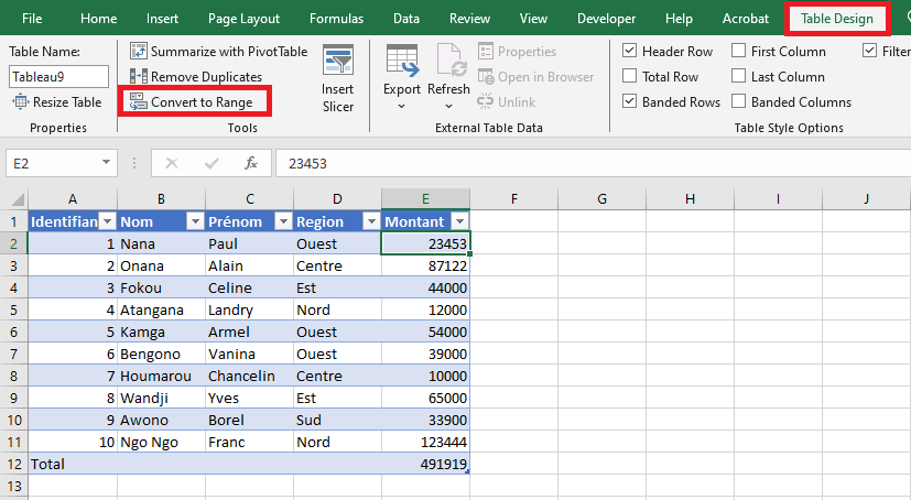
In both cases, Excel will prompt you with a confirmation dialog.
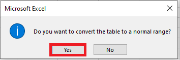
Click Yes to proceed. Once confirmed, the table will be converted to a regular range.
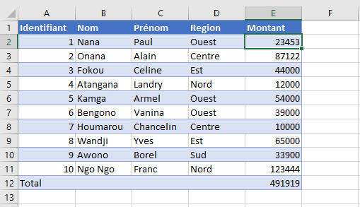
Note that while this process removes table-specific features—such as automatic column expansion, structured formulas, and filter buttons—it preserves the visual formatting (e.g., font colors, cell fill, and borders) applied by the table style.
Converting a Normal Range to an Excel Table
To leverage the full capabilities of Excel tables, you can convert any range of data into a table. There are multiple ways to do this:
- Quick Shortcut Method:
- Select any cell within your data range.
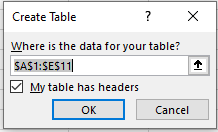
- Press Ctrl + L (or Ctrl + T in newer versions).
-
- In the Create Table dialog box, verify the selected range. If your data includes headers, ensure the My table has headers checkbox is selected.
- Click OK.
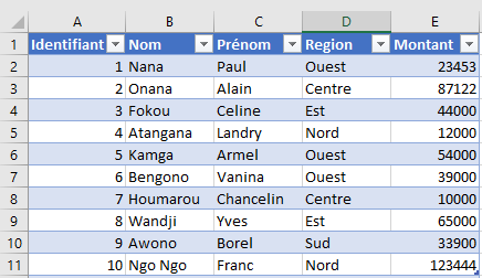
The selected range will instantly become an Excel table, adopting the default table style.
Using the Ribbon to Create a Table
You can also create a table using the ribbon interface:
- Select any cell within your dataset.
- Go to the Insert tab.
- In the Tables group, click Table.
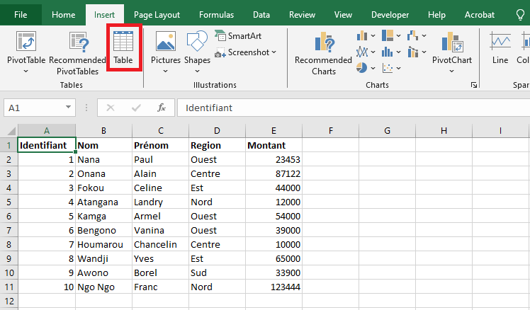
- In the Create Table dialog box, confirm the range and header option, then click OK.
Just like the shortcut method, this action transforms your range into a table with the default style applied.
Converting a Range to a Table with a Specific Style
If you want to apply a specific visual style to your new table right from the beginning, proceed as follows:
- Select any cell within your dataset.
- Navigate to the Home tab.
- In the Styles group, click Format as Table.
- Choose your preferred table style from the gallery.
- In the Create Table dialog, confirm the selected range and whether it contains headers, then click OK.
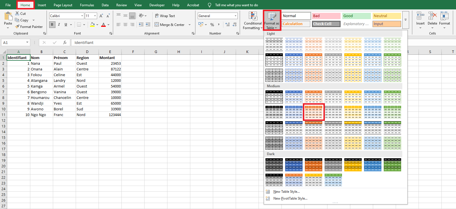
The selected range is now formatted as a table using the chosen style.
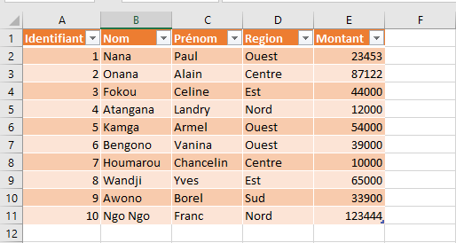
If your dataset already has custom formatting and you want to apply the table style without conflicts, you can right-click the style in the gallery and select Apply and Clear Formatting. This option will remove any existing formatting before applying the table style, ensuring consistency and avoiding design clashes.
- Method 1 (Right-click method):
How to Rename a Table in Excel
Renaming tables in Excel is a best practice that significantly improves the clarity, manageability, and professionalism of your workbooks—especially when dealing with multiple datasets, dashboards, or dynamic reports.
Understanding Excel Table Names
Every table created in Excel is automatically assigned a default name such as
Table1,Table2,Table3, etc. These names are functional but not descriptive, which can make your workbook harder to read, especially when using structured references in formulas or VBA code.Why rename a table?
- To better reflect the content of the table (e.g.,
Sales2024,EmployeeData,Inventory_June) - To make formulas easier to understand
- To avoid confusion when multiple tables exist in the same workbook
- To simplify referencing in Power Query, charts, pivot tables, or macros
Two Main Methods to Rename a Table
Using the Table Design Tab
This method is the most direct and user-friendly.
Steps:
- Click anywhere inside the table to activate the contextual Table Design tab (Excel 2016 and later) or Design tab (earlier versions).
- Look at the left-hand corner of the ribbon, in the group called Properties.

- Locate the field called Table Name.
- Replace the existing name (e.g.,
Table3) with a more descriptive one (e.g.,MonthlyExpenses). - Press Enter to validate the new name.
Tip: If Excel returns an error, it usually means the name is already in use or violates a naming rule (explained below).
Using the Name Manager
This method is more suited for reviewing, managing, and renaming multiple tables and named ranges.
Steps:
- Go to the Formulas tab in the Excel ribbon.
- Click Name Manager in the group called Defined Names.

- In the dialog box, scroll to locate your table (it will appear as
Table1,Table2, etc. under the “Name” column). - Select the table and click Edit.

- In the “Edit Name” dialog, you’ll see:
- Name: enter your desired name (e.g.,
Employee) - Refers to: verify that the correct table range is selected (e.g.,
=Sheet1!$A$2:$E$20)
- Name: enter your desired name (e.g.,
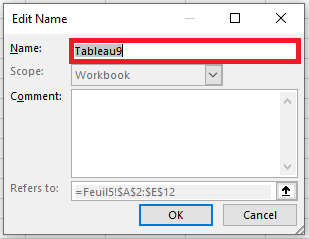
- Click OK, then close the Name Manager.
Note: This method is particularly useful when your workbook contains dozens of named objects, and you need to manage them centrally.
Rules & Conventions for Table Naming in Excel
When renaming tables, you must follow Excel’s strict naming rules. Failing to do so will result in an error message.
Rules:
- Unique names: No two tables can share the same name, even if capitalization differs.
Sales2024andsales2024are treated as identical. - No spaces allowed: Use camel case (
SalesReport2023), underscores (Sales_Report_2023), or hyphens (Sales-Report-2023) to separate words. - Length limit: The name must be 255 characters or fewer, though practical names should ideally stay under 30–40 characters for clarity.
- Valid starting character: Must begin with a letter (A–Z), an **underscore (_) **, or a backslash (\).
After the first character, you may use:- Letters
- Numbers
- Underscores (_)
- Periods (.)
- No cell references: A name like
B3orA1is invalid because Excel could interpret it as a cell reference.
Common Errors When Renaming Tables
Error Cause « That name is already taken » You’ve chosen a name already assigned to another table or named range « The name is not valid » Invalid characters, name too long, or begins with an invalid character Table name turns red You’ve typed an invalid name but haven’t pressed Enter yet
Best Practices for Naming Excel Tables
- Use clear, descriptive names that indicate the table’s purpose (e.g.,
CustomerFeedback_Q1,ProductList_2025) - Prefer camel case (
EmployeeRecords) or underscores (Employee_Records) to improve readability - Avoid special characters like
@,#,!,%,?, etc. - Use consistent naming throughout the workbook for easier navigation and troubleshooting
- To better reflect the content of the table (e.g.,
Anatomy and Features of an Excel Table
An Excel table is a powerful tool for organizing, analyzing, and managing data efficiently. A typical table consists of three main structural components: the header row, the data body range, and the total row. In addition, Excel tables offer advanced features such as calculated columns and a resizing handle. Below is a detailed explanation of each of these elements.
The Header Row
The header row is the topmost row of an Excel table and is typically visible by default. It defines the field names or column headers of your dataset. These headers must be static values (not formulas) to maintain formula references and enable structured references, a key feature in Excel table formulas.
Headers serve two main purposes:
-
They define the identity of each column.
-
They display filter drop-down buttons that provide powerful options to sort and filter data.
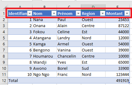
Each header value within a single table must be unique. If you accidentally enter duplicate header names, Excel will automatically append a number to one of them to preserve uniqueness (e.g., entering a second “ID” column will result in “ID2”).
To make headers dynamic, you can use data validation lists, allowing users to choose from a predefined list of possible header names. If a header is changed, all formulas referring to that column automatically update accordingly.
The Data Body Range
This is the central portion of the table, found between the header and the total row. It contains the actual data records. If no data is present, Excel shows a single empty row where data can be entered.
The size of the data body range is only limited by the total number of rows available in the worksheet. The body range grows automatically as you add new entries and is designed to support Excel features like structured referencing, dynamic filtering, and formatting.
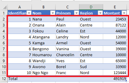
The Total Row
The total row appears at the bottom of the table and is optional. It is hidden by default but can be displayed to provide summary calculations like Sum, Average, Count, Max, Min, etc.
When you select a cell in the total row, a drop-down list appears allowing you to choose a built-in aggregate function. These calculations are automatically adjusted to consider only visible rows, which is useful when filters are applied. You may also insert your own custom formulas, referencing cells inside or outside the table.
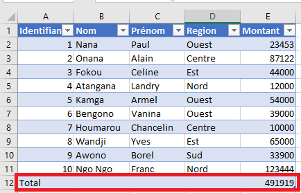
Calculated Columns
A calculated column automatically applies the same formula to all cells in that column’s data range. When you enter a formula into a single cell of a calculated column, Excel automatically propagates it throughout the column, maintaining consistency.
If the column contains a mix of values and formulas, and is not yet recognized as a calculated column, Excel will display an AutoCorrect Options button after formula entry. You can use it to convert the column into a fully calculated one.
Note: There is no built-in indicator to show if a column is truly a calculated column. The best method is to edit a formula and observe whether Excel offers to apply it to the entire column.
The Resize Handle
In the bottom-right corner of the table is a small resize handle, a square icon used to adjust the size of the table. By clicking and dragging this handle, you can expand or shrink the table’s range.
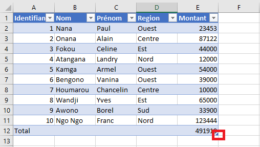
This is useful when adding or removing rows/columns manually. You can also resize the table from the Table Design tab on the ribbon, using the Resize Table option.
Table Behavior and Constraints
Excel imposes several design limitations on tables to preserve functionality:
-
Headers must occupy a single row only.
-
The table can have only one total row.
-
Duplicate column headers are not allowed.
-
Multi-cell array formulas are not permitted (single-cell arrays are allowed).
-
Tables cannot overlap with other tables.
-
Each table must have a unique name within the workbook.
Additionally, you cannot save a workbook with tables in shared mode, although you may publish it via SharePoint for collaborative work.
These rules ensure that Excel can manage structured references, auto-expansion, and dynamic formulas reliably within tables.
Freezing Table Rows
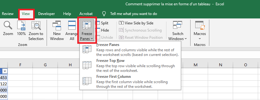
In large tables, identifying columns can become difficult when scrolling down, as the header row disappears from view. To solve this, you can freeze the top row via the ribbon (View > Freeze Panes > Freeze Top Row), ensuring the headers stay visible as you scroll.
When headers aren’t frozen, Excel compensates by temporarily displaying the table’s headers in place of the usual column letters (A, B, C, etc.) when you’re working inside the table.
Accessibility
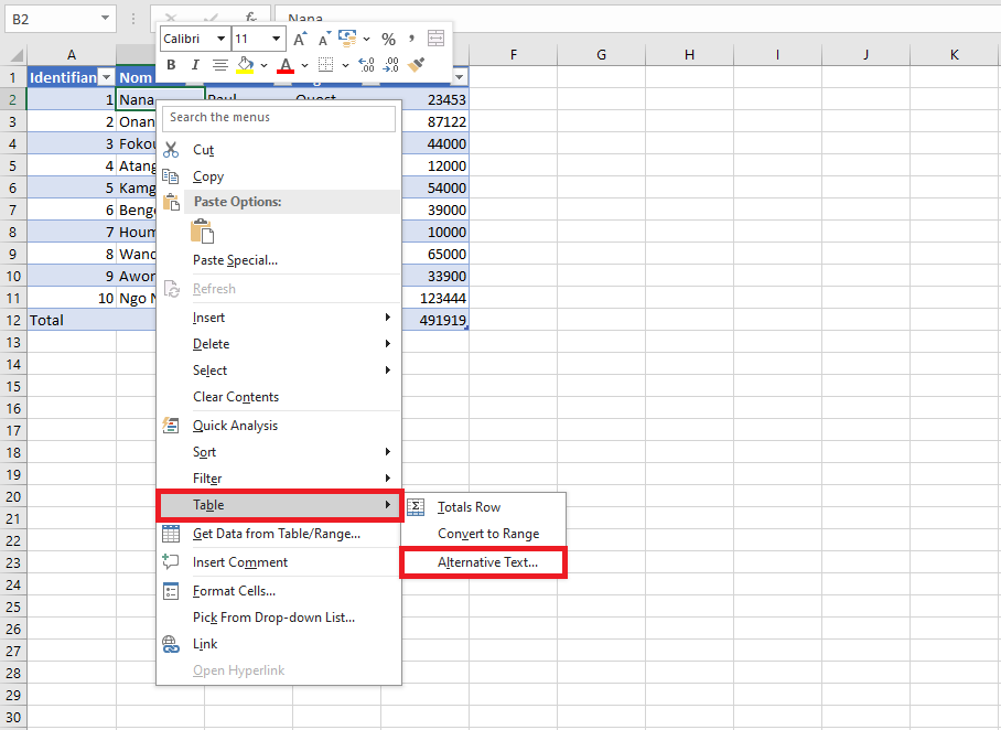
Excel supports alternative text (alt text) for tables, helping users who rely on screen readers and other assistive technologies.
 T
TTo set alt text, right-click on any table cell, go to Table > Alt Text, and fill in the description. This improves accessibility for both web publications and documents exported in formats like DAISY. When users hover over a table with alt text, the description appears as a tooltip.
-
Create an Excel table from a range of cells
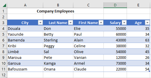
To simplify the management and analysis of related datasets, you can convert a standard cell range into an Excel Table. Despite the generic name, Excel Tables are powerful tools packed with features that make your data easier to organize, analyze, and maintain over time. If you frequently update your datasets or require dynamic formulas that automatically adapt to new entries, then Excel Tables are exactly what you need.
Tables offer functionalities like sorting, filtering, automatic formatting, and more. It is generally recommended to format your data ranges as named Excel Tables to leverage these capabilities and additional advantages outlined below.
Advantages and Disadvantages of Excel Tables
Advantages
- Dropdown menus in header cells make sorting and filtering extremely convenient, allowing users to explore and extract insights quickly.
- Dynamic range: Excel Tables automatically expand or shrink when you add or remove rows, ensuring your data range always reflects the latest updates.
- Built-in styles allow you to quickly format tables for readability or presentation, without manual adjustments.
- Automatic filling of formulas and formatting: When you enter a formula in one row, Excel applies it to the entire column.
- Structured references: Instead of cell coordinates like A2:A10, formulas use column names (e.g., =SUM(Table1[Sales])), improving clarity and interpretability.
- Total row toggle: Easily enable a total row at the bottom of your table to calculate sums, averages, counts, and more without writing manual formulas.
- Seamless integration with PivotTables: Excel Tables are ideal sources for PivotTables, since they automatically adjust to include new data without requiring a manual update of the data source range.
Disadvantages
Despite their benefits, Excel Tables also have limitations, which may influence your decision depending on your workflow:
- Structured references lack absolute referencing, making it more difficult to copy formulas across columns without adjustments.
- Tables do not automatically expand on protected worksheets, even if the cells beneath are unlocked.
- Limitations with worksheet operations: You cannot group, copy, or move multiple sheets if at least one of them contains a table.
- Custom views cannot be created in workbooks that contain one or more Excel Tables.
Preparing Your Data for Table Conversion
Before converting a range into a formatted Excel Table, it is important to properly organize your data:
- Arrange your dataset in rows and columns, where each row represents a unique record (e.g., a customer order or inventory transaction).
- The first row should contain column headers, each with a short, descriptive, and unique title.
- Each column should contain consistent data types: one for dates, another for currencies, another for text, etc.
- Every row should include all the relevant details for a record. Ideally, use a unique identifier (like an order number) to avoid confusion.
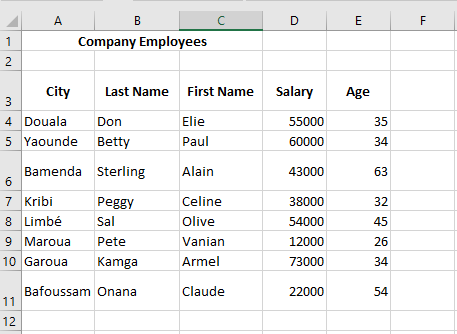
- Avoid empty rows or columns within the list, as they can interfere with Excel’s ability to define the table’s boundaries.
- Keep the dataset isolated from other data on the worksheet, preferably with at least one empty row and column separating it from other content.
Creating an Excel Table
Once your dataset is properly structured, follow these steps to convert it into an Excel Table:
- Select any cell within your dataset.
- Go to the Insert tab on the ribbon.

- In the Tables group, click on the Table command.
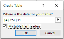
- In the Create Table dialog box, Excel automatically identifies the range of your dataset. Make sure the “My table has headers” option is selected if your first row contains column names.
- Click OK to confirm. Your data is now formatted as an Excel Table.
Creating a Table Using Keyboard Shortcuts
You can quickly insert a table using keyboard shortcuts:
- CTRL + T or CTRL + L: Both shortcuts launch the Create Table dialog box.
- For a guided keyboard navigation: From the Home tab, press ALT, then H, then T, and use the arrow keys to select your desired table style. Press Enter to insert the table.
- From the Insert tab, press ALT, then N, then T to access the table insertion option.
Why CTRL + L?
While CTRL + T seems logical for creating a “Table,” CTRL + L is a legacy shortcut from Excel 2003, where formatted lists (not yet called « Tables ») were created using this shortcut. When Microsoft introduced the Ribbon in Excel 2007, they preserved older keyboard shortcuts (now called “Key Tips” or “Access Keys”) to maintain compatibility. In non-English versions of Excel, CTRL + L is sometimes the only functional shortcut, as CTRL + T may be reassigned to other functions.
Table Design Tools in Excel
After you create a Table, Excel reveals a new contextual ribbon tab labeled Table Design (or Table Tools > Design depending on the version). This tab only appears when a cell within the Table is selected. It gives access to various tools like:
- Changing the table name
- Enabling the total row
- Applying or modifying styles
- Adding banded rows or columns
- Managing table ranges
This dynamic behavior is also shared by other objects such as PivotTables, slicers, charts, and images—each of which activates contextual tabs when selected.
Buttons: « Cancel », « Retry », and « Ignore » in Excel VBA
An example featuring three buttons: CANCEL, RETRY, and IGNORE, accompanied by a warning icon. The associated VBA code is as follows:
Sub MsgBoxAbortRetryIgnore()
    Dim response As Integer
    response = MsgBox("An error occurred during the save process." _
        & vbCrLf & "Do you want to cancel the operation?" _
        & vbCrLf & "Do you want to retry the operation?" _
        & vbCrLf & "Do you want to ignore this message?", _
        vbAbortRetryIgnore Or vbExclamation, _
        "Save Error")
    If response = vbAbort Then
        MsgBox "You chose to cancel the operation."
    ElseIf response = vbRetry Then
        MsgBox "You chose to retry the operation."
    Else
        MsgBox "You chose to ignore the message."
    End If
End Sub
Explanation:
This example demonstrates how to create a message box with three distinct buttons — Cancel, Retry, and Ignore — that allows the user to respond to a critical situation such as an error during a save process. These buttons provide the user with options to either cancel the operation, retry it, or ignore the warning altogether.
The message box also includes a warning symbol (the exclamation mark icon) to clearly indicate the seriousness of the message. When the user clicks one of the buttons, the code detects the choice via the variable
responseand then displays a corresponding confirmation message reflecting the user’s selection.Prompting to Start a New Game in Excel VBA
After successfully completing the puzzle, the user is asked whether they want to start a new game. If the answer is Yes, the procedure
PromptNewGame()is called to begin a new puzzle. Otherwise, the procedureClearBoard()is called to clear the board:Sub PromptNewGame() If MsgBox("Congratulations! Start a new game?", _ vbYesNo, "New Game?") = vbYes Then StartGame Else ClearBoard End If End SubAdditional Tips:
Enjoy playing, exploring the code, and creating your own extensions! For example:
- Provide multiple images and select one randomly for each new game.
- Adjust the number of puzzle pieces (e.g., 3×3, 4×4, 6×6) to control the difficulty level.
- Track time or number of moves to make it competitive.
- Add sound effects or animations for a more dynamic experience.