Votre panier est actuellement vide !
Catégorie : Excel VBA Course
Variable Types in Excel VBA
The data type of a variable specifies the kind of data that the variable can store. You specify the data type of a variable by including the keyword
As. The syntax is as follows:Dim VariableName As Type
If no data type is specified, the default type is Variant. VBA supports the following data types for variables:
Name Type Details Byte Numeric Integer from 0 to 255. Integer Numeric Integer from -32,768 to 32,767. Long Numeric Integer from –2,147,483,648 to 2,147,483,647. Currency Numeric Fixed-point number from –922,337,203,685,477.5808 to 922,337,203,685,477.5807 Single Numeric –3.402823E38 to –1.401298E-45 (negative); 1.401298E–45 to 3.402823E38 (positive) Double Numeric –1.79769313486232E308 to –4.94065645841247E-324 (negative); 4.94065645841247E-324 to 1.79769313486232E308 (positive) String Text Text. Date Date Date and time. Boolean Boolean True or False. Object Object Microsoft object. Variant All Any data type (default if not declared). NOTE
When you find a statement in a VBA procedure that assigns a value to a variable, you can quickly locate the variable’s definition by selecting the variable name and pressing Shift+F2 or choosing View / Definition. Visual Basic jumps to the variable declaration line. Press Ctrl+Shift+F2 or choose View / Last Position to return to the previous cursor location.Boolean Type
You can use the Boolean data type to store Boolean values. Boolean variables can only take two values:
TrueorFalse. A Boolean variable occupies two bytes of space. The declaration is:Dim ProductAvailable As Boolean
A Boolean variable, when converted to another type, returns
-1forTrueand0forFalse. When converting a numeric value to Boolean,0returnsFalseand all other numbers returnTrue.Numeric Data Types
These types are used for mathematical operations such as addition, subtraction, multiplication, etc. For example: percentage calculation, stock price, fees, invoices, age, etc. In VBA, there are six numeric data types:
- Byte, Integer, and Long for integer values
- Single and Double for decimal values
- Currency for monetary values
NOTE
When you declare a variable as an integer type (e.g., Long) and assign it a decimal number, no error occurs, but only the integer part is retained.More than a decade ago, memory optimization was important. Today, with increasingly powerful computers, such concerns are obsolete. You can use Long for all integers and Double for all decimals.
Date Type
You can use the Date data type to store a date. Each Date variable occupies eight bytes. The range for Date is from January 1, 0100 to December 31, 9999, and the time from 0:00:00 to 23:59:59.
Dates must be enclosed in hash signs (
#) when assigned:MyDate = #6/5/01# MyDate = #June 6, 2001#
VBA converts the literal date into the
mm/dd/yyyyformat. You can also assign a time similarly.Object Type
An object variable refers to an entire object, like a Range or Worksheet. These variables are important because:
- They simplify your code.
- They speed up execution.
The
Objectdata type can hold references to any object. However, it’s preferable to declare variables as the specific object type they reference:Dim GenericObj As Object Dim SpecificObj As Worksheet
GenericObjcan reference any object.SpecificObjcan only reference aWorksheet.
Using
Objectis called late binding, meaning the object type isn’t known until runtime, which disables IntelliSense and slows performance slightly.Using a specific type is called early binding, enabling IntelliSense and helping you write code faster.
Declaring a specific object type doesn’t initialize it. Example:
Dim mySheet As Worksheet
Set mySheet = Worksheets("Sheet6")
Use the
Setkeyword when assigning an object reference. You may also need to use theNewkeyword:Set ObjectVar = New ObjectType Dim ObjectVar As New ObjectType
Without Object Variable:
Sub NoObjectType()
    Worksheets("Sheet3").Range("C4").Value = "ELIE"
    Worksheets("Sheet3").Range("C4").Font.Size = 16
    Worksheets("Sheet3").Range("C4").Font.Name = "Verdana"
    Worksheets("Sheet3").Range("C4").Font.Bold = True
    Worksheets("Sheet3").Range("C4").Font.Italic = True
End Sub
With Object Variable:
Sub WithObjectType()
Dim myRange As Range Set
     myRange = Worksheets("Sheet6").Range("C4")
     myRange.Value = "ELIE"
     myRange.Font.Size = 16
     myRange.Font.Name = "Verdana"
     myRange.Font.Bold = True
     myRange.Font.Italic = True
End Sub
String Type
Use the
Stringtype when your variable holds text. Strings are enclosed in quotation marks.Dim myVar As String myVar = "This is a string"
By default, strings are variable-length. You can also declare fixed-length strings:
Dim myVar As String * 50
This sets the string length to exactly 50 characters. Extra characters are truncated; shorter strings are padded with spaces.
VBA supports only concatenation as a string operation, using
&or+. Prefer&to avoid confusion:Dim x As String x = "Visual Basic " & "for Applications"
Variant Type
The
Varianttype is the default for undeclared variables. You can declare it explicitly:Dim myVar As Variant
Variants can hold strings, dates, booleans, or numbers and automatically convert between types. Numeric variants need 16 bytes; string variants need 22 bytes plus character storage. Due to memory usage, prefer explicitly declaring types.
User-Defined Types (UDT)
A user-defined type (UDT) lets you group different data types into a single structure. You define it using the
Typestatement, usually at the top of the module:Type ClientInfo Company As String Phone As Long City As String POBox As Long Income As Double End TypeDeclare an array of this type:
Dim Clients(1 To 20) As ClientInfo
Access individual fields:
Clients(5).Company = "CESTAD ANALYTICS"
Clients(5).Phone = 699072798
Clients(5).City = "Douala"
Clients(5).POBox = 15652
Clients(5).Income = 17598000
Limitations:
- Cannot instantiate dynamically.
- Cannot validate fields.
- UDTs are static structures.
Use classes to overcome these.
Identifying Variable Types
Use
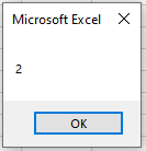
VarType()to determine the data type of a variable:Sub TestVariables() firstName = "chancelin" MsgBox VarType(firstName) age = 33 MsgBox VarType(age) End SubReturns
8(String), then2(Integer).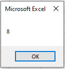
Value Type Return Value Variant 0 Null 1 Integer 2 Long 3 Single 4 Double 5 Currency 6 Date/Time 7 String 8 Boolean 11 Byte 17 If you perform math on a non-numeric Variant, you get a Type Mismatch error.
Functions to Test Variable Values
Numeric Value
UseIsNumeric()to test if a Variant holds a number:Sub TestNumeric() name = "chancelin" MsgBox IsNumeric(name) End SubReturns
False.Date/Time Values
Date/time values are floating-point numbers. The integer part represents days since Dec 31, 1899; the decimal part represents time.Example:
37786.75= June 14, 2003, at 6:00 PM.Use
IsDate()to check for a date:Sub TestDate() myDate = "01-Feb-2002" MsgBox IsDate(myDate) End SubReturns
True.Empty Value
UseIsEmpty()to check if no value has been assigned:MsgBox IsEmpty(MyTest)
Returns
True.Null Value
A Variant can contain a special valueNull, representing unknown or missing data. UseIsNull()to test for it.Return Values
The table below lists constants returned by
VarType():Constant Value Description vbEmpty 0 Variable is uninitialized. vbNull 1 No valid data. vbInteger 2 Integer vbLong 3 Long integer vbSingle 4 Single vbDouble 5 Double vbCurrency 6 Currency vbDate 7 Date vbString 8 String vbObject 9 Object reference vbError 10 Error code vbBoolean 11 Boolean vbVariant 12 Variant (only for arrays of variants) vbDataObject 13 Non-ActiveX object reference vbDecimal 14 96-bit scaled real vbByte 17 Byte vbLongLong 20 LongLong (64-bit only) vbUserDefinedType 36 User-defined type vbArray 8192 Array value Shorter Variable Declarations
Advanced programmers may use abbreviations:
Detailed Shorthand Dim Client As IntegerDim Client%Dim MainClient As LongDim MainClient&Dim Amount As CurrencyDim Amount@Dim ClientInfo As StringDim ClientInfo$You can also use naming conventions to suggest data type, e.g.:
str_messagefor a stringi_SalesJanuaryfor an integer
Variables (Declaration and Scope) in Excel VBA
A variable can simply be a single number, a piece of text, or a series of information that the program needs to retain and refer to during its execution. The program can change the value of a variable during its execution. That is why it is called a variable. If a variable has been defined as a given type, data specified as a different type will not be accepted. For example, if you define a variable as an integer, you cannot insert text into it.
Variable Declaration
To create a variable, you must declare it, that is, assign it a name that can then be reused to operate on the value stored in it. Variable declaration in VBA can be implicit or explicit. In other words, VBA programs can recognize a new variable without it being previously created in a declaration statement. You can also configure the Visual Basic Editor to require explicit variable declaration before use.
You can assign any name you like to a variable, as long as it follows these rules:
- It must begin with a letter.
- It cannot contain more than 255 characters.
- Periods, exclamation points, spaces, and the characters @, &, $, and # are not allowed.
- The variable name must not be a reserved word, meaning a word recognized as part of the Visual Basic language (function name, object, property, argument, etc.).
NOTE
Uppercase and lowercase letters are considered identical in variable names.Implicit Declaration
It is not necessary to declare a variable before using it. You can simply include the statement:
DeclaVaria = 10
A variable will automatically be created for
DeclaVariaas a Variant type (default type) and will have the value 10.Variable types will be presented later in this chapter.
However, the problem is that this can lead to subtle errors in your code if you misspell the variable name in a later statement. For example, if you refer toDeVariainstead ofDeclaVaria, you know what you mean, but VBA does not. It assumesDeVariais a new variable and assigns it as such. The old variableDeclaVariastill exists but is no longer used. You now have two different variables, although you think you only have one. This can cause major issues that may take a long time to correct in your code.Explicit Declaration
To avoid the issue of incorrect variable names, you can require VBA to always generate an error message whenever it encounters an undeclared variable.
To force variable declaration before use, add the
Option Explicitstatement. Its use helps prevent errors due to typos in variable names. To do this, place yourself in the Declarations section of the module’s Code window and type theOption Explicitstatement, as shown in the following figure.
From now on, the appearance of variable names not previously declared using the
Dimstatement will generate an error, as in the figure.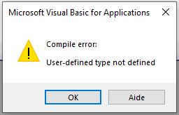
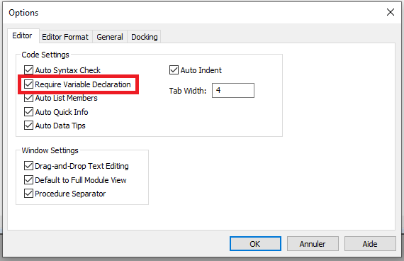
You can also configure the Visual Basic Editor to automatically insert the
Option Explicitstatement in the Declarations section of every new module. Here’s how:- Select the Options command from the Tools menu and go to the Editor tab.
- Check the box Require Variable Declaration, then click OK, as shown in the figure.
The method you use (implicit or explicit) depends on your personal preferences. Coding is often much faster with implicit declaration because you don’t need to define your variables beforehand. You can simply use them, and VBA will handle the rest. However, as mentioned earlier, this can lead to errors unless you have a good memory for the variables you use and the experience to know exactly what you are doing. Implicit declaration can also make it harder for someone else to understand your code. Using
Option Explicitis the best practice and helps prevent runtime errors.Declaring a Variable with the Dim Statement
Variable declaration is done using the
Dimstatement with the following syntax:Dim VariableName As Type
Comments
- The
Dimstatement (short for Dimension) defines a name as a variable and allocates storage space for it. VariableNameis the name chosen for this variable.- The
Askeyword declares the data type. - The
Typeargument represents the data type and can be values likeLong(integer),Double(decimal),String(text type)… It is optional, but specifying a type often saves memory and improves program performance.
You can declare several variables on a single line:
Dim MyVar1, MyVar2, MyVar3 As Long
In this example,
MyVar1andMyVar2are declared as Variant (the default type in VBA), and onlyMyVar3is declared as Long. Why? Because Excel VBA requires that each variable’s type be declared explicitly, even if they’re on the same line (unlike C or many other languages). To declare all three variables as Long, the correct syntax is:Dim MyVar1 As Long, MyVar2 As Long, MyVar3 As LongVariable Scope and Lifetime
All procedures, functions, variables, and constants in VBA have their own scope. This means they can only be used in a specific area of the program’s code, precisely where they are defined.
For example, if variable
Ais defined in the body of a procedure namedProcedure1(), then that procedure is its scope. So, if another procedureProcedure2()exists, you cannot use the same variable name in it. If you try, you will either get an error (ifOption Explicitis active), or you will simply have another variable with the same name, unrelated to the first one.There are three types of variable scope:
- Procedure-level scope: Variables declared with
DimorStaticinside a procedure are recognized only within that procedure. These are called local variables. - Module-level scope: Variables declared using
DimorPrivateoutside of any procedure, in the declarations area of a module, can be used throughout that module only. - Project-level scope: Variables declared with the
Publickeyword at the module level are available to all procedures in the project. These are called public variables.
A variable declared with
Privateretains its value only during the execution of the procedure where it is defined. After the procedure ends, its value is lost. When the procedure runs again, the variable is reinitialized. However, variables declared withStaticretain their value after the procedure ends and while the program continues running.Let’s examine the scope of procedures and functions.
Procedures and functions only have two levels of scope: module-level and project-level. The default is project-level. Therefore, a procedure or function can be called by any other procedure or function in the project. The optional
Publickeyword can also be used for project-level procedures. Its presence or absence has no effect on behavior.If you want a procedure to be used only within the current module, use the
Privatekeyword. Note that this not only restricts the procedure’s scope but also prevents it from being used as an independent procedure—it can only be called from another procedure.Finally, the
Statickeyword can be used with procedures or functions. It does not affect the scope but affects all variables declared within it. In this case, all local variables retain their values after the procedure ends and preserve them when called again.Example:
Public B1 As String
Private B2 As Integer
Dim B3 As Single
Sub Procedure1()
   Dim B4 As Integer
   Static B5 As Integer
   B1 = "Un texte"
   B2 = 2
   B3 = 3.14
   B4 = B4 + 4
   B5 = B5 + 5
   MsgBox B4
   MsgBox B5
End Sub
Sub Procedure2()
   Procedure1
   MsgBox B1
   MsgBox B2
   MsgBox B3
   MsgBox B4
   MsgBox B5
   Procedure1
End Sub
Comments
- In this example,
B1is defined at the project level (withPublic),B2andB3at the module level,B4at the procedure level (inProcedure1()), andB5is defined asStaticwithinProcedure1(). - When
Procedure2()is called, it first callsProcedure1(), which assigns values to all five variables and displays the values ofB4andB5. - Once
Procedure1()ends,Procedure2()displays the current values of all five variables. VariablesB1,B2, andB3retain their values since they are declared at the project or module level. VariablesB4andB5, having procedure scope, are empty—each procedure uses its own variables even if they share names. - When
Procedure1()is called again, the values ofB4andB5are updated and displayed.B4is reset to 4, since it is reinitialized with each call, butB5, being static, retains its previous value, and is incremented to 10.
The Excel VBA Macro Recorder
The Excel VBA Macro Recorder
The easiest way to create a macro is to record your worksheet actions using a valuable tool called Record Macro. All you have to do is turn on the macro recorder, perform the actions that make up the task you want to automate, then turn off the recorder once you’re done. While the macro recorder is active, every action you perform—selecting a cell, entering a number, formatting a range, almost anything—is recorded and represented as VBA code in a new macro. As you’ll see later, when you run the macro created by the recorder, your task is executed automatically as if you had done it manually.
The macro recorder is useful for repetitive common tasks that you’d prefer not to do manually.Create Your First Macro Using the Macro Recorder
Let’s suppose we need to create a macro that activates a worksheet. So, if we have Sheet1 active, we will write a macro to activate worksheet Sheet2.
- Start Microsoft Excel and make sure the cell pointer is on Sheet1.
- To activate the macro recorder, go to the Developer tab on the ribbon, and in the Code group, click Record Macro.

In the Record Macro window that opens, set the required parameters for the recorded procedure: for example, assign the name
ActivateSheet2to the macro, enter appropriate explanations in the Description field, and leave the Store macro in field unchanged. Click OK.
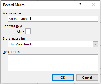
The Macro Name and Description fields are used to specify the macro’s name and its description. A macro name must not contain spaces, and the description is important for reusable macros, as over time it becomes difficult to remember why a given macro was created. By default, macros are named Macro1, Macro2, etc. To facilitate macro recognition, it’s better not to use a standard name but a unique one that describes its purpose.
In last Figure, notice the small box next to Ctrl+ in the Shortcut key section. You can place any letter of the alphabet in this field, and when pressed with the Ctrl key, it becomes a handy way to run the macro.
A shortcut key is not mandatory; in fact, most of your macros won’t need one. But if you choose to assign one, it’s best to use Ctrl+Shift+Key rather than just Ctrl+Key. Excel has already assigned Ctrl plus the 26 letters of the alphabet to built-in shortcuts for various tasks, and it’s best not to override them. For instance, Ctrl+C copies text. However, if you assign Ctrl+C to your macro, you will override the default function and lose the ability to use Ctrl+C to copy text in that workbook.
To use the shortcut key option, click the Shortcut Key field, press Shift, then a letter like S. You’ve now created the shortcut Ctrl+Shift+S, which won’t interfere with Excel’s main shortcuts.The Store macro in dropdown allows you to select the workbook where the macro will be saved. If you select Personal Macro Workbook, the macro will be saved in a special hidden workbook where macros are stored. This workbook is always open but hidden, and the macros in it are available for other workbooks. To view your personal macro workbook, go to the View tab, and in the Window group, click Unhide.
If you select This Workbook (the default choice), the macro is stored in the active workbook. If you select New Workbook, it will be saved in a new workbook.- While recording the macro, go to Sheet2 (the pointer is on cell A1).
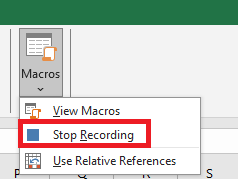
Click the Stop Recording button in the Code group under the Developer tab to stop recording the macro.6.
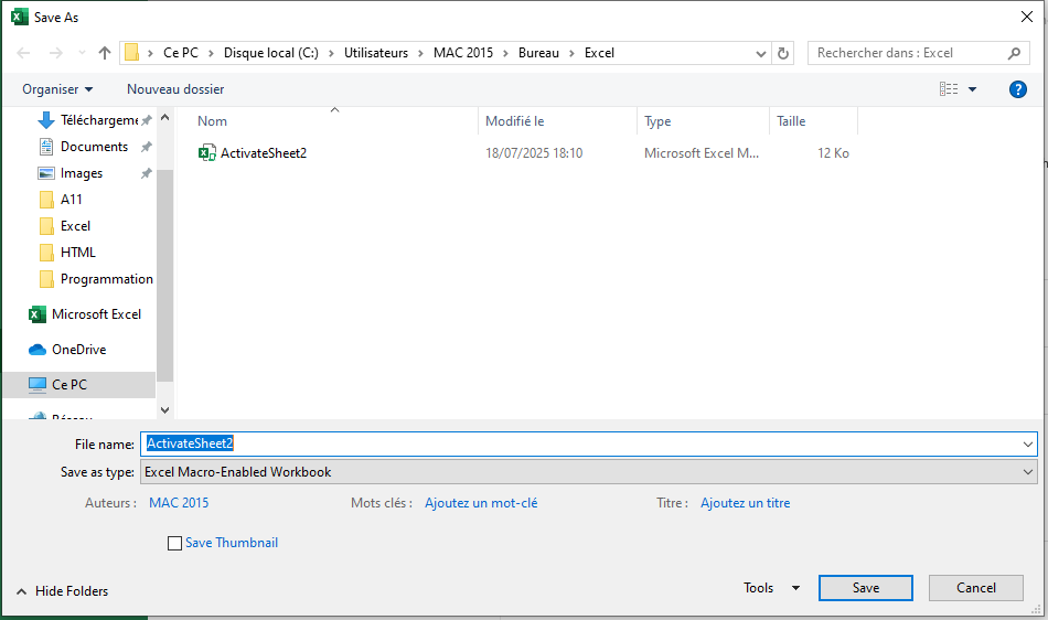
- Save your workbook in a format that supports macros: go to the File tab on the ribbon and select Save As. In the Save As dialog box (Figure 4), choose a save location, enter the workbook
name, and in the Save as type dropdown, choose Excel Macro-Enabled Workbook. Click Save.
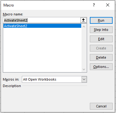
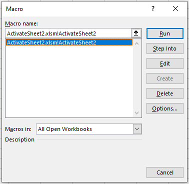
- Go to the Developer tab, click the Macros button in the Code group, and in the Macro window that opens, select your macro from the list (Figure 5) and click Edit.
The screen displays the VBA Editor with the standard module containing the macro code just recorded:
Sub ActivateSheet2()
'
' ActivateSheet2 Macro
'
   Sheets("Sheet2").Select
End Sub
Notes
- A macro starts with the
Substatement and ends withEnd Sub. We’ll go deeper into macro structure in later chapters. ActivateSheet2()is the macro name.- The instruction
Sheets("Sheet2").Selectis the macro body.
Now, without closing this workbook, create another workbook by going to the File tab, selecting New, and choosing Blank Workbook.
- Go to the Developer tab and click Macros in the Code group.
In the Macro window (Figure 6), specify the name of the macro you created and click Run. Ensure that this macro activates Sheet2 in your workbook.
Assigning a Created Macro to a Button
Now let’s assign our created macro to a button placed on the Quick Access Toolbar. Follow these steps:
- Right-click on the Quick Access Toolbar and select More Commands… (Figure 7)
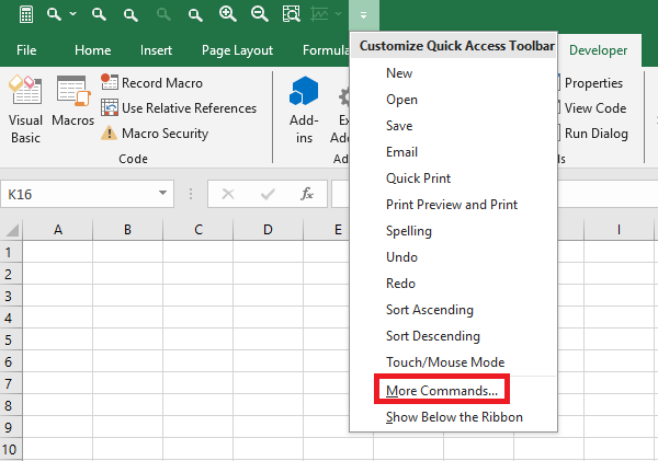
In the Excel Options window that opens, in the Quick Access Toolbar category, select Macros from the Choose commands from dropdown list .
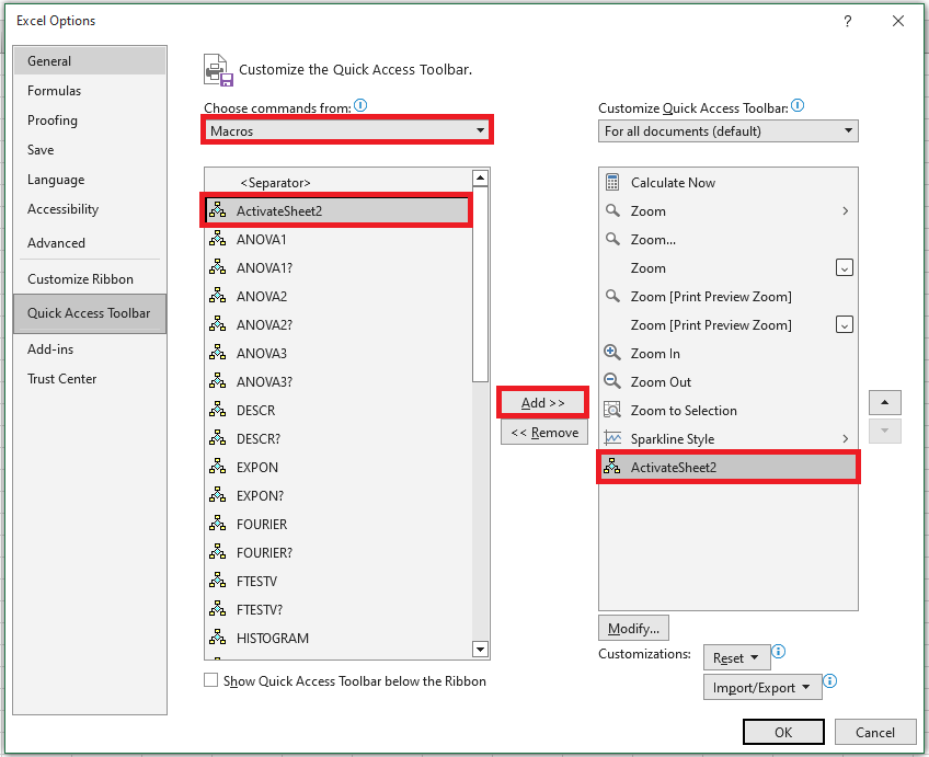
Select the macro
ActivateSheet2that you created in the left column and use the Add >> button to move it to the right column. Note that the Modify button is now available at the bottom of the right column—it’s used to assign an icon to the corresponding macro. Click the Modify button.- In the Modify Button window that opens (Figure 9), choose a symbol for the button using your mouse and, if needed, in the Display Name field, edit the macro name. This display name will appear as a tooltip in the Quick Access Toolbar. Click OK.
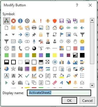
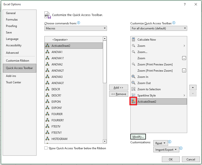
- In the Excel Options window under the Quick Access Toolbar category, the macro button appears in the right column (Figure 10). Click OK.
- Make sure the button with the recorded macro appears in the Quick Access Toolbar.

Automating Worksheet Tasks with Controls
Excel also includes a complete set of controls—command buttons, text boxes, checkboxes, etc.—that you can place on a worksheet if needed. To view the available controls, go to the Developer tab, and in the Controls group, click the Insert button.
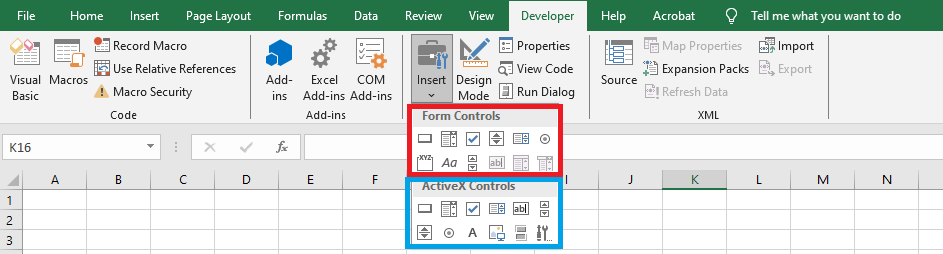
Note: the controls under the Form Controls group are primarily intended for compatibility with files from older Excel versions (up to Excel 97) that use these controls. They are much more limited in capability than the ActiveX Controls. Some of these form controls cannot be used at all in recent Excel documents (text box, list box, combo box). However, these controls have advantages not found in ActiveX controls—for example, they can be placed on chart sheets.
ActiveX controls are standalone components from various applications and can also be used in Microsoft Excel. This group includes controls similar to many in the Form Controls group (UserForm).
In addition to standard controls, you can use extra controls. Excel comes with several of these, such as multimedia controls that let you play sound or video directly from the worksheet. You can also connect controls from other programs or use custom-built controls.
In the worksheet module, you can create procedures that handle events triggered by these controls—for example, pressing a button, selecting a list item, checking an option box, etc. These actions can automatically trigger calculations, build charts, change chart types, and more.
Using a Command Button Control on a Worksheet
We’ll demonstrate how to use an ActiveX Command Button on a worksheet. Suppose that when we click the button, placed on Sheet1, Sheet2 is activated.
- Start Excel and make sure the cell pointer is on Sheet1.
- Go to the Developer tab, and in the Controls group, click the Insert dropdown list.
- Click on the Command Button (ActiveX Control) and move directly to the worksheet—your pointer turns into a thin cross.
Select a location on the worksheet, press the left mouse button, and while holding it, draw the button to the required size. Then release the button.
Note that once the Command Button appears on the sheet, Design Mode is activated.
On the first button’s surface, the default label CommandButton1 is automatically displayed (Figure 14). If you create a second Command Button now, it will be labeled CommandButton2, and so on.
NOTE:
Like any graphical object, a button can be drawn while holding Shift to give it a square shape, or Alt to snap it to the worksheet grid. With the sizing handles, you can adjust its dimensions, and with the move handle, you can set its position.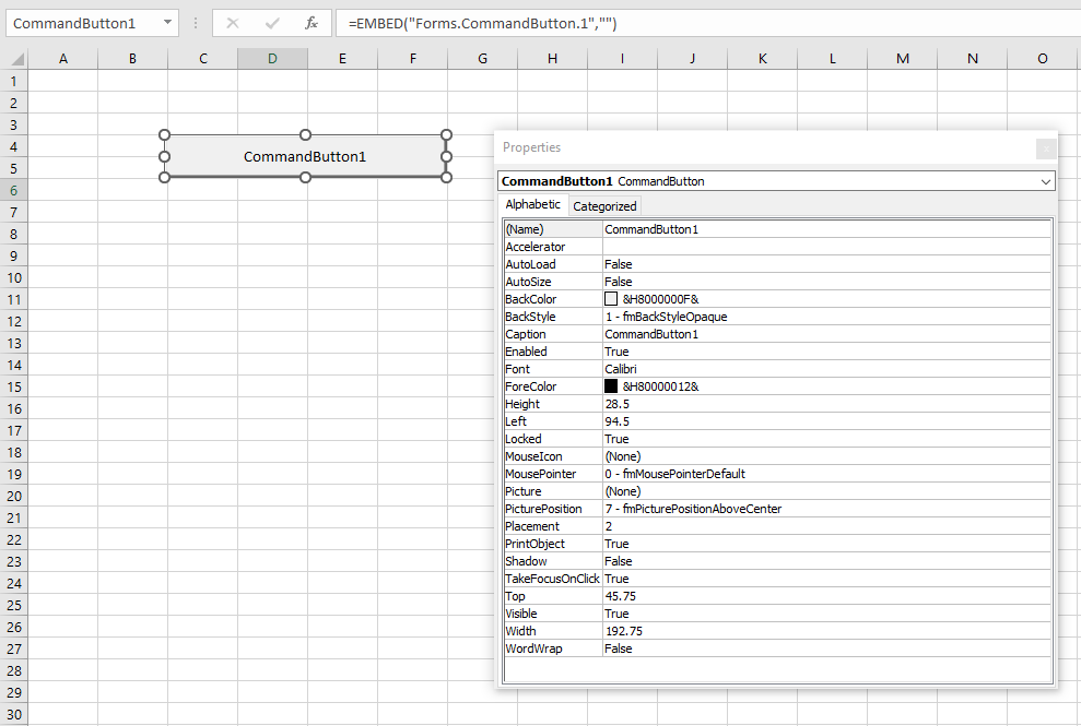
Right-click the created Command Button and in the context menu, select Properties to open the Properties window (see Figure 14). The Command Button is an object, meaning it has properties, methods, and events.
The Caption property sets the name displayed on the button surface. The Name property identifies the object in code. In this case, it’s also CommandButton1. In the Properties window, change the Caption from « CommandButton1 » to Sheet2 (to indicate that this button activates Sheet2). Optionally, test other properties: BackColor, Font, ForeColor, Shadow. Finally, close the Properties window.
- We’ll now write the procedure to handle the Click event. When the event is triggered, Sheet2 will be activated.
Double-click the created Command Button (ensure Design Mode in the Developer tab is still active). This opens the VBA editor with the worksheet module for Sheet1, and automatically adds the starting and ending lines of the event procedure:
Private Sub CommandButton1_Click()
End Sub
- Open the Windows file where you created the
ActivateSheet2macro. Make sure the required module is displayed in the VBAProject – Project Explorer window. - Copy the macro’s line into the clipboard:
Sheets("Sheet2").SelectOf course, you could manually type it, but that’s slower and risks typos. Now insert that line inside the event procedure:
Private Sub
   CommandButton1_Click()
   Sheets("Sheet2").Select
End Sub
Return to Sheet1. The button works only when Design Mode is off. So, click Design Mode in the Controls group on the Developer tab to deactivate it.
8. Test the created Command Button: click it. If everything was done correctly, it will activate Sheet2.Another Example Using the Macro Recorder
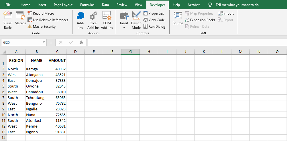
Suppose you manage a data table daily, such as the one shown in the following figure, which displays the number of items sold by your company in its East, West, North, and South regions.
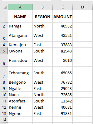
The daily task consists of sorting the table primarily by region, then by item. Your boss wants the columns NAME and REGION to switch places, so that REGION appears in column A and NAME in column B. To improve readability, the numbers in the AMOUNT column must be formatted with a comma separator, and the headers for REGION, NAME, and AMOUNT must be bolded. Next Figure16 shows the finished table, as requested by your boss.
This is normally a six-step process, which is quite tedious but part of your professional responsibilities.
NOTE
Whenever you create a macro, it’s a good idea to plan ahead: think about why you’re creating the macro and what you want the macro to do. This is especially important for complex macros, as you want your code to be efficient and accurate, using only the instructions necessary to get the job done properly. Avoiding excessive code will result in macros that run faster and are easier to edit or troubleshoot. For instance, prepare your workbook in advance to avoid recording unnecessary actions. Make sure the worksheet you’re working on is active and the relevant range is visible.
To complete the task, proceed as follows:
- Insert a new column at column A.
- Select the REGION column, cut it, and paste it into the new column A, to the left of NAME.
- Delete the now-empty column where REGION was.
- Select the range A1:C13 and sort in ascending order by REGION, NAME, and AMOUNT.
- Select range C2:C13 and format the AMOUNT values with a thousands separator.
- Select range A1:C1 and apply bold formatting to the headers.
These steps are not only repetitive but prone to human error. The good news is, if you perform the steps correctly while recording the macro, the task can be reduced to a single mouse click or keyboard shortcut, with VBA doing the heavy lifting for you.
To record the macro that performs this task, follow these steps:
- Start the macro recorder: go to the Developer tab on the ribbon and in the Code group, click Record Macro.
- In the Record Macro dialog box, enter
"FormatData"in the Macro name field, select This Workbook for Store macro in, then click OK. - Now perform the six steps listed above.
- Stop the macro recorder by clicking Stop Recording in the Code group on the Developer tab.
As a result, the following macro will be written to a standard module:
Sub FormatageDonnees()
' FormatageDonnees Macro
' Data Formatting

    Columns("A:A").Select
    Selection.Insert Shift:=xlToRight, CopyOrigin:=xlFormatFromLeftOrAbove

    Columns("C:C").Select
    Selection.Cut
    Columns("A:A").Select
    ActiveSheet.Paste

    Columns("C:C").Select
    Selection.Delete Shift:=xlToLeft

    Range("A1:C13").Select
    ActiveWorkbook.Worksheets("Sheet1").Sort.SortFields.Clear
    ActiveWorkbook.Worksheets("Sheet1").Sort.SortFields.Add Key:=Range("A2:A13"), _
        SortOn:=xlSortOnValues, Order:=xlAscending, DataOption:=xlSortNormal
    ActiveWorkbook.Worksheets("Sheet1").Sort.SortFields.Add Key:=Range("B2:B13"), _
        SortOn:=xlSortOnValues, Order:=xlAscending, DataOption:=xlSortNormal
    ActiveWorkbook.Worksheets("Sheet1").Sort.SortFields.Add Key:=Range("C2:C13"), _
        SortOn:=xlSortOnValues, Order:=xlAscending, DataOption:=xlSortNormal

    With ActiveWorkbook.Worksheets("Sheet1").Sort
        .SetRange Range("A1:C13")
        .Header = xlYes
        .MatchCase = False
        .Orientation = xlTopToBottom
        .SortMethod = xlPinYin
        .Apply
    End With

    Range("C2:C13").Select
    Selection.NumberFormat = "#,##0"

    Range("A1:C1").Select
    Selection.Font.Bold = True
End Sub
Comments
- As seen before, all macros begin with a
Substatement (short for Subroutine, commonly known as a macro), which includes the macro name followed by parentheses. - The comments you see in a recorded macro reflect the information entered in the Record Macro dialog box. For example, if you assign a shortcut key or enter a description, these appear as comments in the code.
- The remaining lines are VBA instructions representing every action performed while recording the macro.
Here’s a breakdown:
- You selected column A.
- You inserted a new column.
- You selected column C, cut it, and pasted it into column A.
- You selected the now-empty column C and deleted it.
- You selected range A1:C13 (the data table).
- You sorted the data.
- You selected C2:C13 to format the numbers.
- You applied a thousands separator.
- You selected A1:C1 for the headers.
- You bolded the font in those cells.
- You stopped the macro recording, which ends with
End Sub.
Improving the Recorded Macro
It’s easy to generate a macro with the Record Macro button. However, the recorded macro often lacks efficiency and produces unnecessary code. To be fair, the Record Macro tool isn’t designed to write optimized code. Its purpose is to produce VBA code that mirrors your on-screen actions exactly.
There’s no rule that says you must always clean up your recorded macros. For simple tasks that work as intended, keeping them as-is can be perfectly fine.
However, for most recorded VBA code, the unnecessary and inefficient parts can’t be ignored. Moreover, if you plan to share your VBA work, you’ll want it to look clean and professional.
A key VBA development principle is: Avoid
SelectandActivateunless necessary. These are often the main reason for slow-running macros.For example, these two recorded lines:
Columns("A:A").Select
Selection.Insert Shift:=xlToRight
Can and should be simplified to:
Columns("A").Insert Shift:=xlToRightSimilarly, this code:
Columns("C:C").Select
Selection.Cut
Columns("A:A").Select
ActiveSheet.Paste
Can be replaced with:
Columns("C").Cut Destination:=Columns("A")And this code:
Columns("C:C").Select
Selection.Delete Shift:=xlToLeft
Can be simplified to:
Columns("C").Delete Shift:=xlToLeftBy streamlining the code, your
FormatDatamacro becomes more readable and much more efficient.The VBA editor
Introduction to the Visual Basic Editor (VBE) in Excel
It is fair to say that for many Excel users, worksheets, pivot tables, charts, and hundreds of formula functions are all the tools they need to satisfactorily manage their spreadsheet activities. For them, the familiar workbook environment is the only aspect of Excel they see, and it is obviously the only aspect of Excel they are likely aware of.
But Excel has a separate, less visible environment working behind the scenes called the VBE (Visual Basic Editor), which is interconnected with the workbook environment even if no programming code exists in the workbook. The two environments constantly but quietly work together, sharing information about the workbook as a whole. The Visual Basic Editor is a user-friendly development environment where programmed instructions are stored to make your spreadsheet applications work.How to Launch the Visual Basic Editor
The VBE icon is found in the Developer tab of the ribbon. By default, the Developer tab is not automatically displayed with the other ribbon tabs. Use the following steps to make the Developer tab visible:
■ Click on the File tab, then click the Options button as shown in Figure. The Options dialog box opens.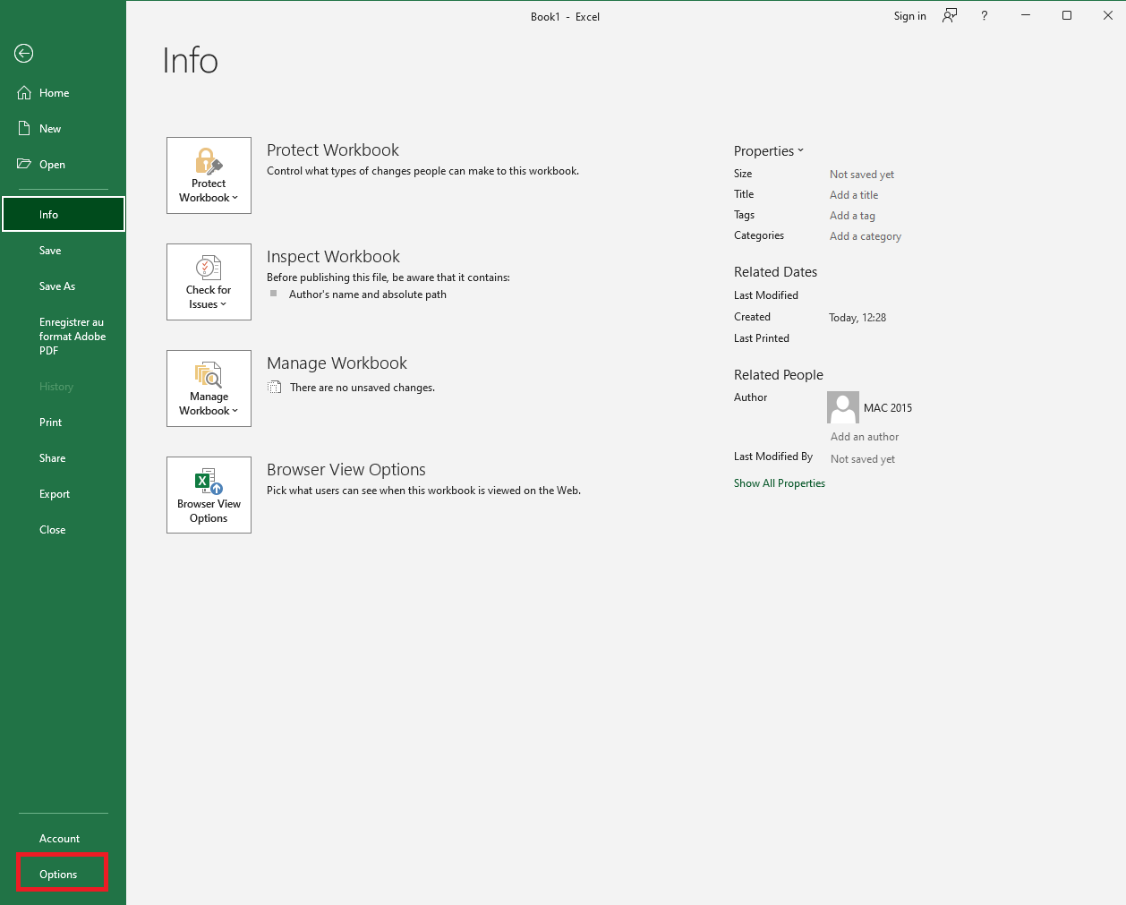
■ Click on the Customize Ribbon item on the left, which displays two vertical lists, as shown in Figure 2. Note that the list on the right has a dropdown menu above labeled Customize the Ribbon.
■ Select the Main Tabs item in the Customize the Ribbon dropdown list.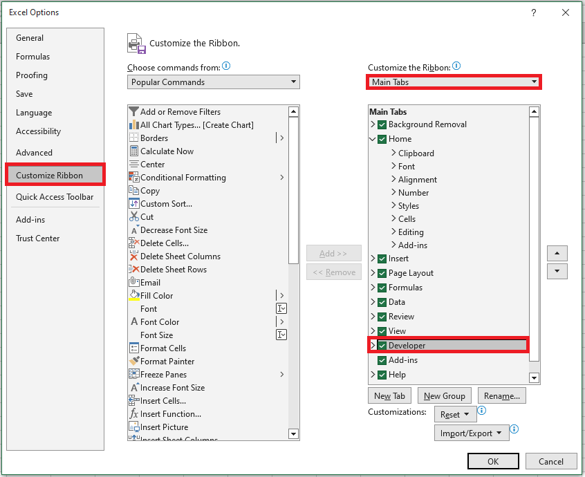
■ In the list of Main Tabs, select Developer and click OK. You will now see the Developer tab in your ribbon, as illustrated in Figure.
To finish, click on the Visual Basic button in the Developer tab of the ribbon, as shown in Figure.

Another quick and easy way to access the Visual Basic Editor is by pressing Alt + F11 on your keyboard. You can do this from any worksheet.
NOTE:
The Alt + F11 keyboard shortcut allows you to access the Visual Basic Editor in all versions of Excel.Main Windows of the VBE
The Visual Basic Editor can display a number of different windows, depending on what you want to see or do. For most tasks, you should become familiar with four windows: the Project Explorer window, the Code window, the Properties window, and the Immediate window. Figure 1.5 shows what the VBE looks like with these four windows.
Figure 1.5 The four main VBE windowsThe Project Explorer Window
The Project Explorer window is a vertical pane on the left side of the VBE. It displays a hierarchical list of currently open projects and their elements. A VBA project may contain the following elements:
■ Worksheets
■ Chart sheets
■ ThisWorkbook: the workbook in which the project is stored
■ Modules: special sheets where programming code is stored
■ Classes: special modules that allow you to create your own objects
■ Custom Forms (UserForms)
■ References to other projectsYou can activate the Project Explorer window in three ways:
■ From the View menu, select Project Explorer.
■ From the keyboard by pressing Ctrl + R.
■ From the Standard toolbar by clicking the Project Explorer button.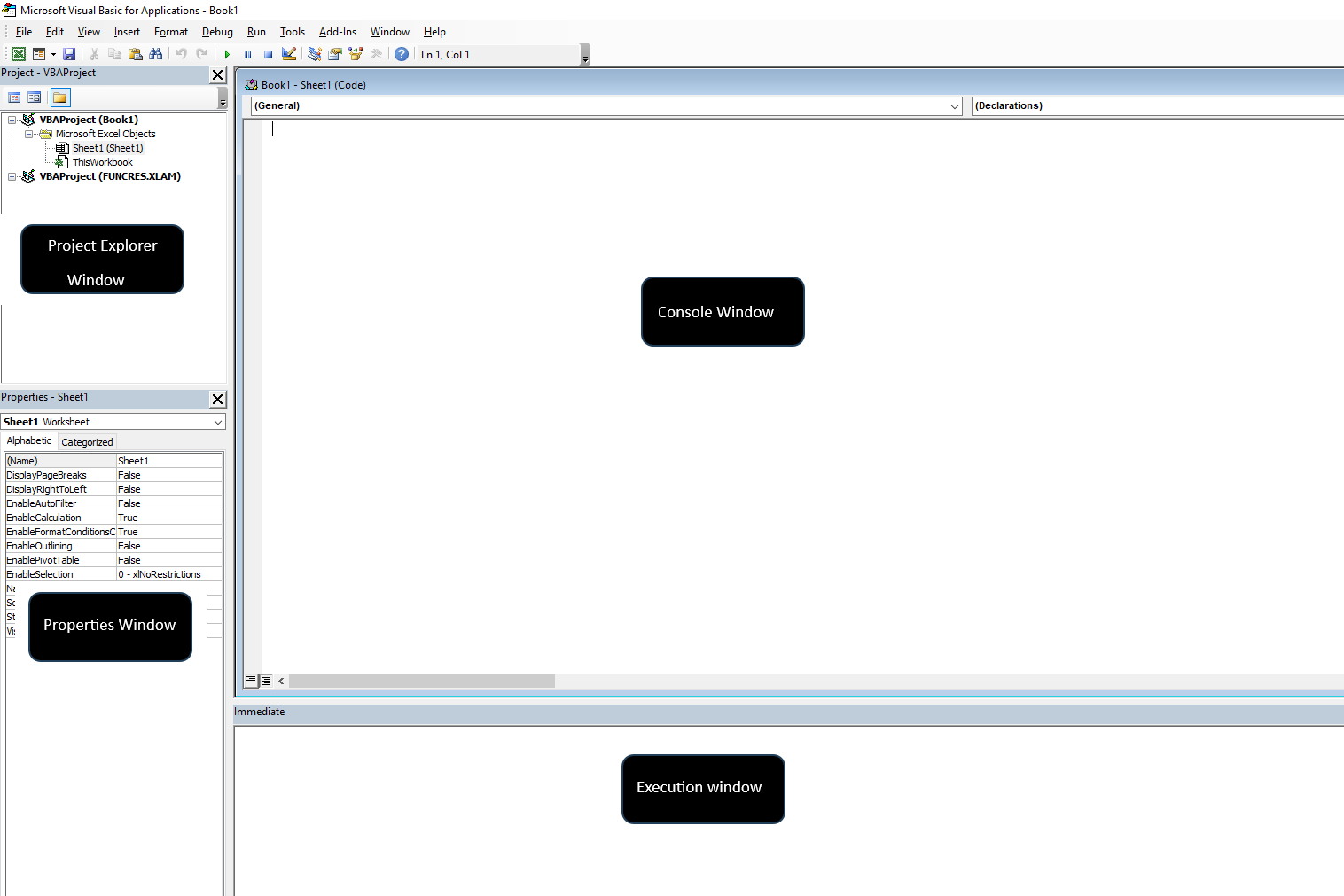
The Code Window
The Code window is used for Visual Basic programming and for viewing and editing recorded macros and existing VBA procedures. Each module can be opened in a separate Code window. There are several ways to activate the Code window:
■ In the Project Explorer window, select the appropriate UserForm or module, then click the View Code button.
■ In the menu bar, choose View | Code.
■ On the keyboard, press F7.The Code window is made up of several parts:
■ The code input area
■ Two dropdown lists at the top of the Code window, allowing you to quickly navigate through your Visual Basic code
■ The margin indicator bar used by the VBE to display helpful markers during editing and debugging
■ Two icons at the bottom-left of the Code window:- Procedure View displays one procedure at a time in the Code window
- Full Module View displays all procedures in the selected module
The Properties Window
The Properties window is located in the lower part of the left vertical pane of the VBE. It allows you to view and set properties for various objects in your project. Object properties can be viewed alphabetically or by category by clicking the appropriate tab:
■ Alphabetic Tab: Lists all properties of the selected object in alphabetical order.
You can modify a property’s setting by selecting the property name and typing or selecting the new value.
■ Categorized Tab: Lists all properties of the selected object by category.
You can collapse the list to view categories or expand a category to see its properties. The plus (+) sign to the left of a category name indicates that the list can be expanded. The minus (–) sign means the category is currently expanded.The Properties window can be accessed in three ways:
■ From the View menu, select Properties Window.
■ From the keyboard by pressing F4.
■ From the toolbar by clicking the Properties Window button.The Immediate Window
The Immediate window is located at the bottom of the VBE, usually below the Code window, as shown in Figure 5.
The Immediate window is used to try out various instructions, functions, and operators present in the Visual Basic language before using them in your own VBA procedures. The Immediate window allows you to type VBA statements and immediately test their results without writing a full procedure. The Immediate window is like a notepad. Use it to test your statements. If the instruction produces the expected result, you can copy it from the Immediate window into your procedure.
If you do not see the Immediate window in your VBE, press Ctrl + G or, in the VBE menu bar, click View → Immediate Window.
To close the Immediate window, click the Close button in the upper-right corner of the window.Introduction
What is VBA?
VBA is a programming language created by Microsoft to automate operations in Excel. In addition to Excel, VBA can also manipulate other Microsoft Office applications such as Access, Word, PowerPoint, and Outlook. It is an extremely powerful tool that allows you to control many methods in Excel that you cannot or do not want to do manually. VBA is the tool you use to develop macros and manipulate objects to control Excel and other Office applications from within Excel. You do not need to purchase anything other than the Office suite to also have VBA. If you have Excel on your computer, then you have VBA on your computer.What is a “macro”?
VBA is therefore a programming language, and it is also a macro language. Terminology confusion arises when referring to VBA code, which is a series of commands written and executed in Excel. So, what is a macro? A macro can be described as a sequence of instructions written in the VBA language that are stored in a module. When we call a macro, by pressing a button or using a key combination, the instructions stored in it are triggered.
With macros, we can not only streamline tasks that we perform frequently, but we can also extend Excel’s functionality by creating new functions to solve calculations that cannot be performed with the program’s standard functions.
There are two ways to create a macro. One uses the Record Macro tool, and the other involves writing the instructions directly in the Visual Basic Editor built into Excel. Since Excel 2007, Microsoft has distinguished between saving a workbook with macros (file extension .xlsm) and a workbook without macros (file extension .xlsx).There is a big difference between VB and VBA!
With all the acronyms circulating in the world of computing, it’s easy to confuse certain terms. VB means Visual Basic, and it is not the same as VBA.
Although both VB and VBA are programming languages derived from BASIC and created by Microsoft, they are otherwise very different.
VB is a language that allows you to create executable, standalone applications that do not even require users to have Office or Excel installed on their computers.
VBA, on the other hand, cannot create standalone applications. It can only exist within a host application such as Excel and the workbook that contains the VBA code. For a VBA macro to run, its host application’s workbook must be open.
This book is based on VBA and how it controls Excel.What can you do with VBA?
Everyone reading this book uses Excel for their own purposes, such as financial budgeting, forecasting, scientific data analysis, creating invoices, or tracking the progress of their favorite soccer team. One thing all readers have in common is the need to automate some frequently encountered task that takes too much time or is too cumbersome manually. This is where VBA comes into play.
Many VBA commands are at your disposal and are relatively easy to implement and customize for your daily needs.
Anything you can do manually, you can do with VBA — but VBA allows you to do it faster and with a reduced risk of human error.
Many things that Excel doesn’t allow you to do manually can be done using VBA. Here are a few examples of what VBA can do for you:- Automate a recurring task: If you need to produce weekly or monthly sales and expense reports, a macro can create them in no time. And if the source data changes later in the day and you need to generate the updated report again — no problem, just rerun the macro!
- Automate a repetitive task: When you need to perform the same task on every worksheet in your workbook or in every workbook in a particular folder, you can create a macro to loop through each object and perform the action.
- Automatically run a macro when another action occurs: In some cases, you want a macro to run automatically so you don’t have to remember to run it yourself. For example, to automatically refresh a PivotTable when its source data changes, you can monitor those changes with VBA, ensuring your PivotTable always displays real-time results. This is called event-driven programming.
- Create your own worksheet functions: You can create your own worksheet functions, called User Defined Functions (UDFs), to handle custom calculations that Excel’s built-in functions do not support.
- Create full-scale applications driven by macros:
If you’re willing to invest the time, you can use VBA to create large-scale applications with a custom Ribbon tab, dialog boxes, screen tips, and many other features. - Create custom Excel add-ins:
You’re probably familiar with some of the add-ins that come with Excel — for example, the Analysis ToolPak is a popular one. You can use VBA to develop your own add-ins for specific purposes.
Sorting Data by Multiple Columns in Excel
As you continuously add content to your spreadsheet, keeping the data organized becomes increasingly important. One of the most effective ways to manage this is by sorting your data. Sorting allows you to rearrange the contents of your sheet to make it easier to analyze or find specific information. For instance, you can sort a contact list alphabetically by last name or sort numerical values in ascending or descending order. Excel offers multiple sorting options, including single-column, multi-column, and even custom or horizontal sorts.
Types of Sorting
Before applying a sort, it’s essential to determine whether you want to sort the entire worksheet or just a specific range of cells:
-
Worksheet Sort: This applies the sort to all rows, keeping data in each row together. It’s useful for entire datasets where each row represents a record.
-
Range Sort: This applies sorting only to a selected portion of the worksheet. It’s ideal when you’re working with multiple tables on a single sheet and only need to sort one of them without affecting the others.
Sorting an Entire Worksheet (Example: by Last Name)
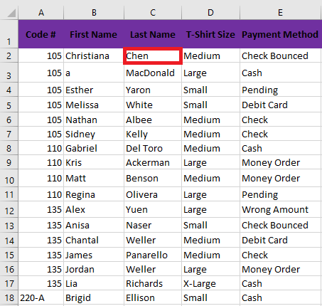
To sort a full dataset alphabetically by a column (e.g., Last Name in Column C):
-
Click a cell in the column you want to sort (e.g., C2).
-
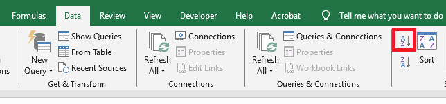
Go to the Data tab and click either A to Z (ascending) or Z to A (descending).
-
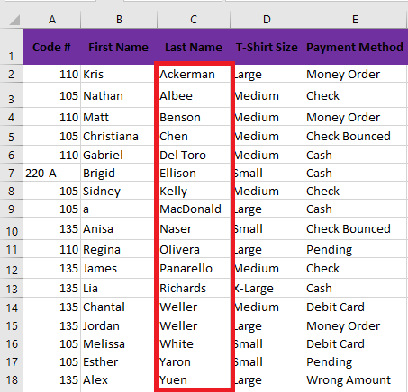
The sheet will be sorted based on the selected column. All rows will adjust accordingly to maintain data integrity.
Sorting a Range Only (Example: by Number of T-Shirts Ordered)
To sort a selected range (e.g., G2:H6) by the number of T-shirts:
-
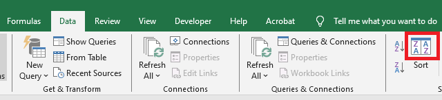
Highlight the range of cells you want to sort.
-
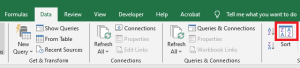
Click the Sort command in the Data tab.
-
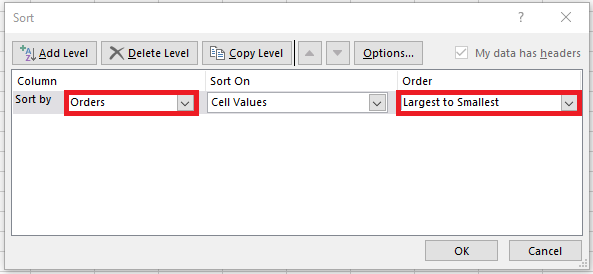
In the Sort dialog box, choose the column to sort by (e.g., « Orders »).
-
Specify the sort order (e.g., Largest to Smallest).
-
Click OK. Only the selected range will be sorted—other parts of the worksheet remain unchanged.

If sorting doesn’t work correctly, double-check for typing errors or inconsistent data formats (e.g., text vs. numbers).
Custom Sorting (Using a Custom List)
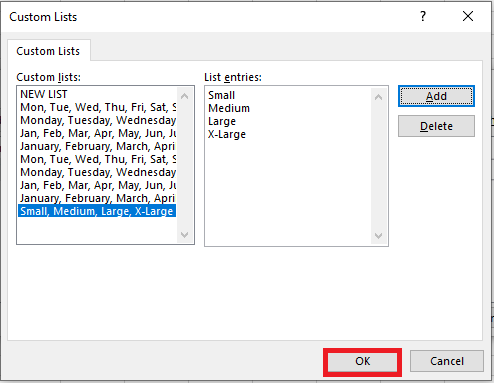
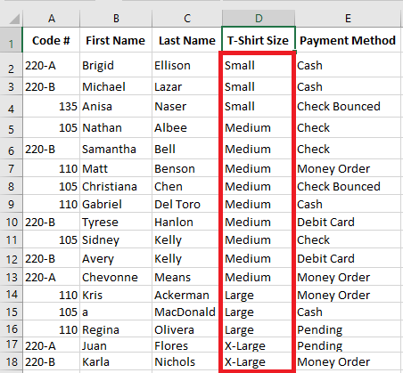
Default sorting in Excel (alphabetical or numerical) may not always suit your needs. When sorting items like T-shirt sizes (Small, Medium, Large, X-Large), alphabetical sorting is inappropriate. Here’s how to apply a custom sort order:
-
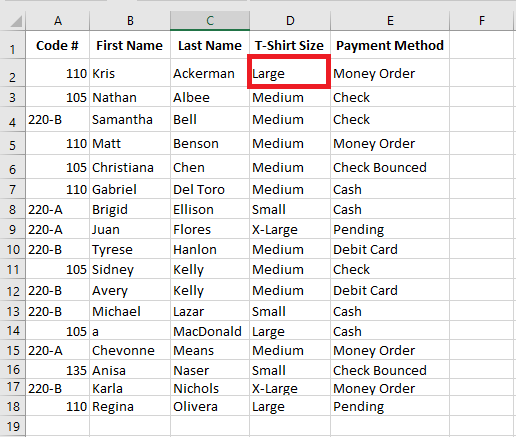
Select a cell in the target column (e.g., D2 for T-shirt sizes).
-
Click Sort in the Data tab.
-
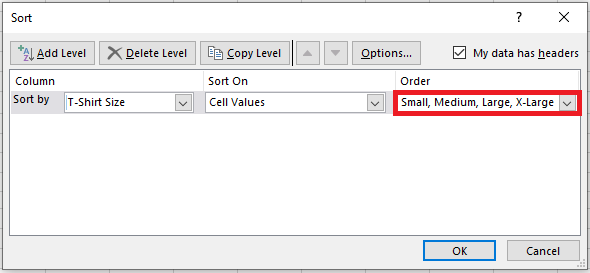
In the Sort dialog, choose the relevant column, then under “Order”, click Custom List.
-
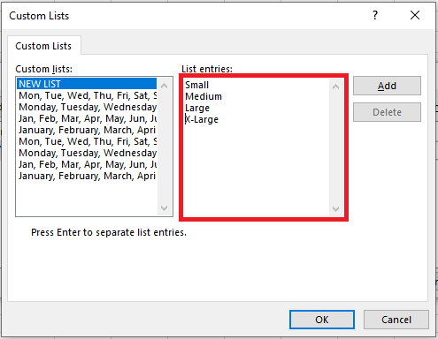
In the Custom Lists window, select New List and type your custom sequence (e.g., Small, Medium, Large, X-Large), pressing Enter after each entry.
-
Click Add then OK to apply the sort.
-
Click OK again in the Sort dialog. Your data will now be sorted according to the custom list.
Multi-Level Sorting (Sorting by Multiple Columns)
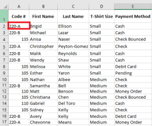
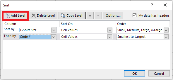
To gain more control, you can sort data based on multiple criteria (e.g., first by T-shirt size, then by order code):
-
Select any cell in your dataset.
-
Click Sort on the Data tab.
-
In the Sort dialog:
-
Set the first level (e.g., « T-shirt Size ») and choose the custom list as the order.
-
Click Add Level, then define the second level (e.g., « Order Code »).
-
-
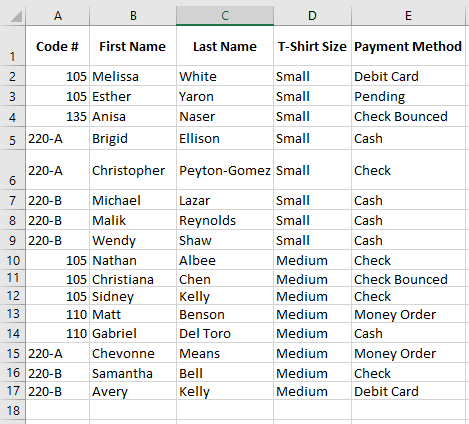
Click OK to apply. Excel will first group data by size, then within each group, sort by code.
Sorting Horizontally (By Rows Instead of Columns)
Although most Excel sorts are vertical (by columns), you can also sort horizontally—i.e., rearranging columns based on values in a particular row. This is useful in non-traditional layouts like side-by-side comparisons.
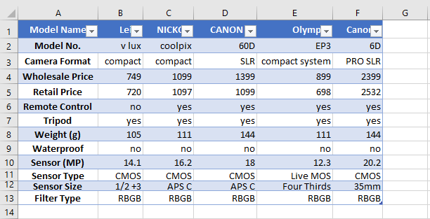
Example: You want to sort camera models based on their names (row 1) or prices (row 4):
-
Select the data range (e.g., B1 to F5). Avoid selecting the first column (A) if it contains feature labels.

-
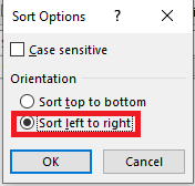
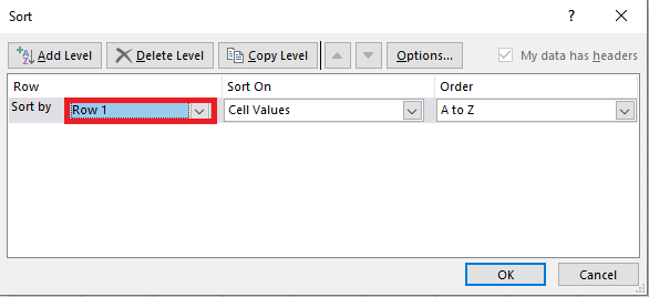
Go to Data > Sort, then click Options in the Sort dialog.

-
In Sort Options, choose Sort left to right, then click OK.
-
Back in the main Sort dialog:
-
Under “Sort by,” select the row to use (e.g., Row 1 for model names or Row 4 for prices).
-
Choose sort order (A to Z or Smallest to Largest).
-
-
Click OK. Excel will rearrange entire columns based on the selected row’s values.
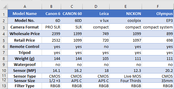
Excel preserves data integrity by moving full columns rather than individual cells.
Note: This horizontal sorting method can be used to sort by any critical parameter—image sensor size, camera weight, resolution, etc.—depending on your specific need.
-
Filtering Records in Excel
When your spreadsheet contains a large amount of data, it can become challenging to quickly locate the information you need. Excel’s filtering feature allows you to refine your data view by displaying only the rows that meet specific criteria. Below is a comprehensive guide to using filters effectively in Excel.
Applying Basic Filters
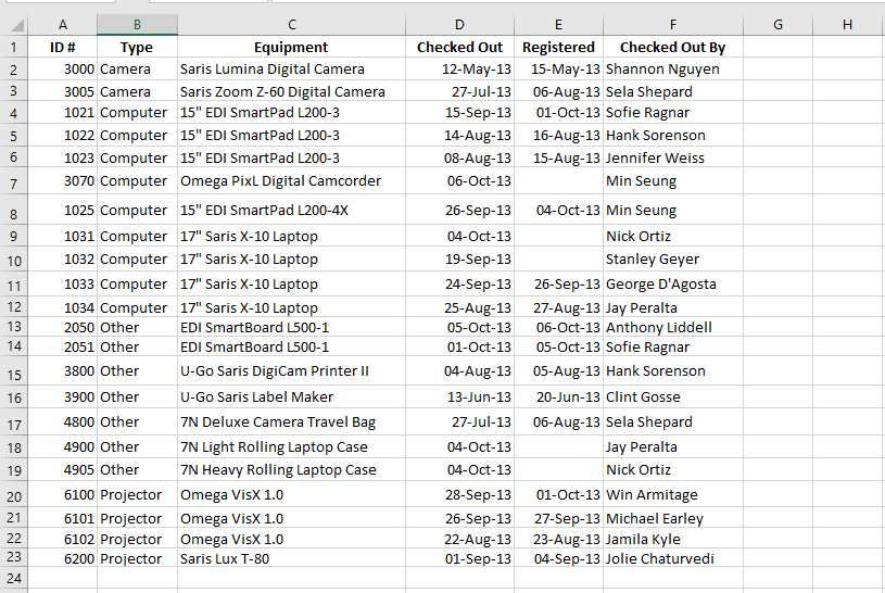
In this section, we’ll apply a filter to an equipment log spreadsheet to display only laptops and projectors that are available for payment.
-
Ensure your spreadsheet has a header row. This row (usually the first) contains labels for each column such as ID#, Type, Equipment, etc. These labels are required for Excel to identify which fields to filter.
-
Go to the Data tab and click the Filter command.

-
A dropdown arrow will appear next to each header cell.
-
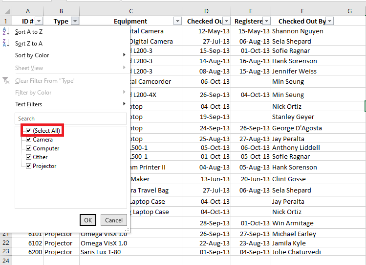
Click the dropdown arrow in the column you wish to filter. For instance, filter Column B to display only specific equipment types.

-
The filter menu will appear.
-
Uncheck “Select All” to quickly deselect everything.
-
Then, check only the options you wish to display — in this example, “Laptop” and “Projector”. Click OK.
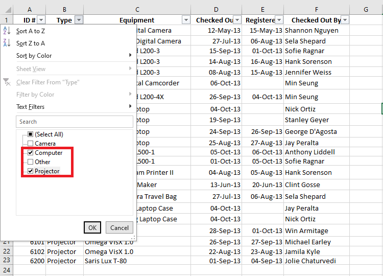
-
Excel will now hide all rows that do not match the selected values, making only laptops and projectors visible.
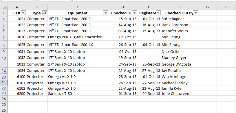
You can also access filtering options via the Home tab under the “Sort & Filter” group.

Applying Multiple Filters
Excel allows cumulative filtering, meaning you can apply multiple filters across different columns to narrow down results even further.
Let’s say the sheet is already filtered to show only laptops and projectors, and now you want to display only those items that were checked out in August:
-
Click the dropdown arrow in the Date column (e.g., Column D).
-
The filter menu appears.
-
Deselect all other months except August, then click OK.
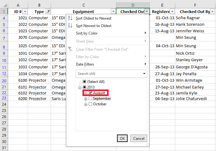
-
Your spreadsheet will now show only laptops and projectors that were checked out in August.
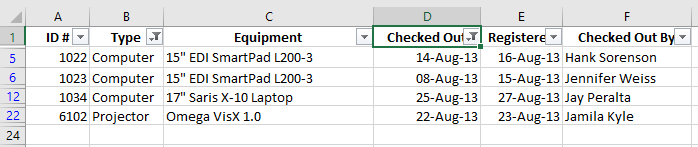
Clearing Filters
Once you’re done analyzing, you may want to remove filters:
-
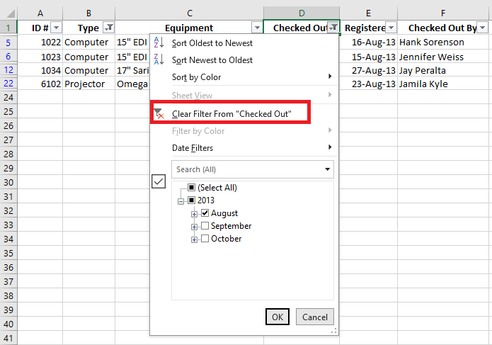
Click the dropdown arrow of the filtered column (e.g., Column D).
-
Choose Clear Filter From [Column Name].
-
All previously hidden rows will reappear.
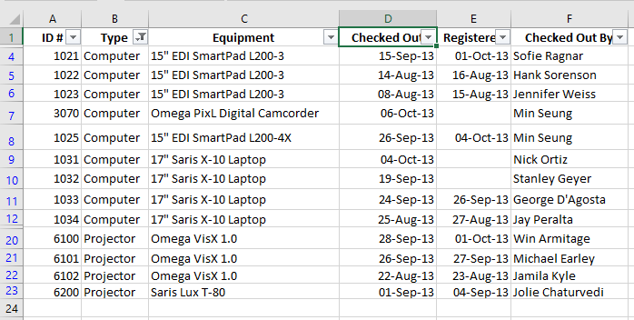
To remove all filters in one click, go to the Data tab, click on the Filter command, and then choose Clear.

Using Advanced Filtering Options
If basic filters aren’t sufficient, Excel provides advanced filtering tools like search, text filters, date filters, and number filters to help pinpoint specific data.
Filtering with the Search Box
Let’s say you want to view only equipment from the brand “Saris”:
-
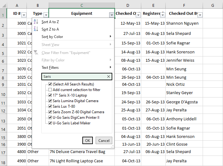
Click the dropdown arrow in the Brand column (e.g., Column C).
-
In the search box, type Saris.
-
Excel will dynamically display matching options. Select them and click OK.
-
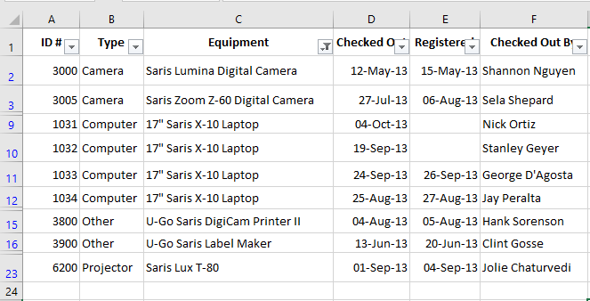
The sheet will now show only rows containing the brand “Saris”.
Using Advanced Text Filters
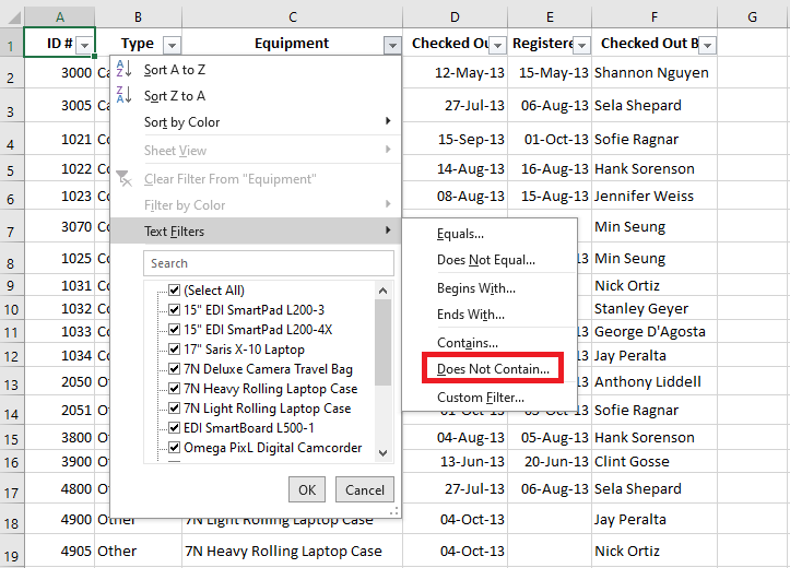
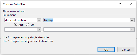
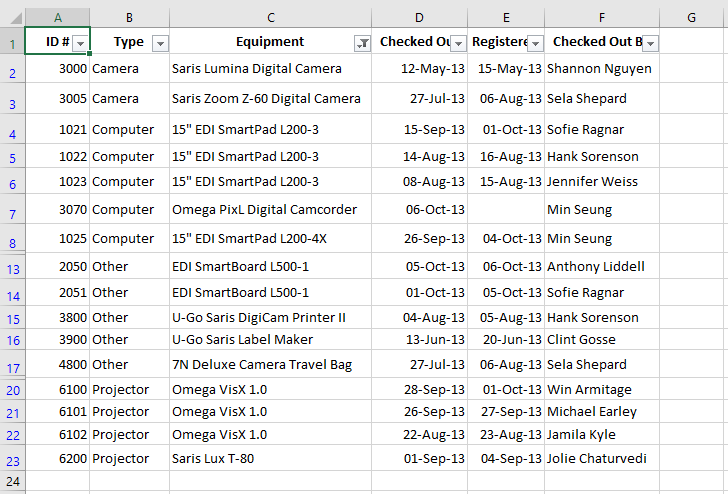
Text filters allow for even more control. For example, to exclude all items containing the word Laptop:
-
Click the dropdown arrow in Column C.
-
Hover over Text Filters and select Does Not Contain…
-
In the dialog box, type Laptop and click OK.
-
The filtered view will now exclude any item that contains the word “Laptop”.
Using Advanced Number Filters
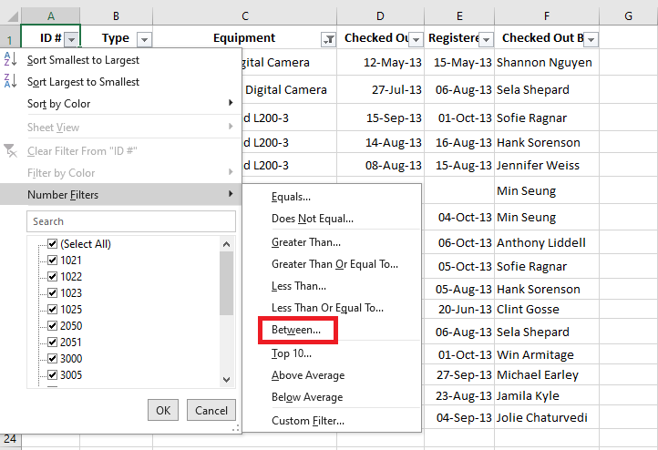
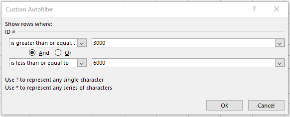
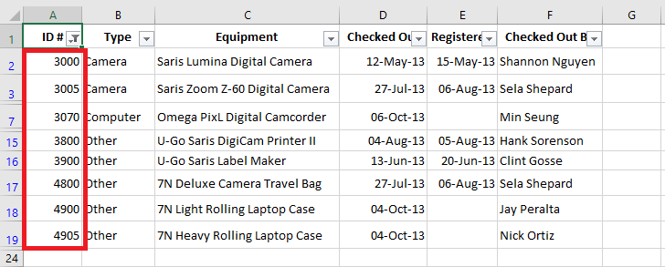
To display equipment with ID numbers between 3000 and 6000:
-
Click the dropdown in the ID# column (A).
-
Hover over Number Filters, and choose Between…
-
Enter 3000 and 6000, then click OK.
-
Excel will now display only items with IDs in the specified range.
Using Advanced Date Filters
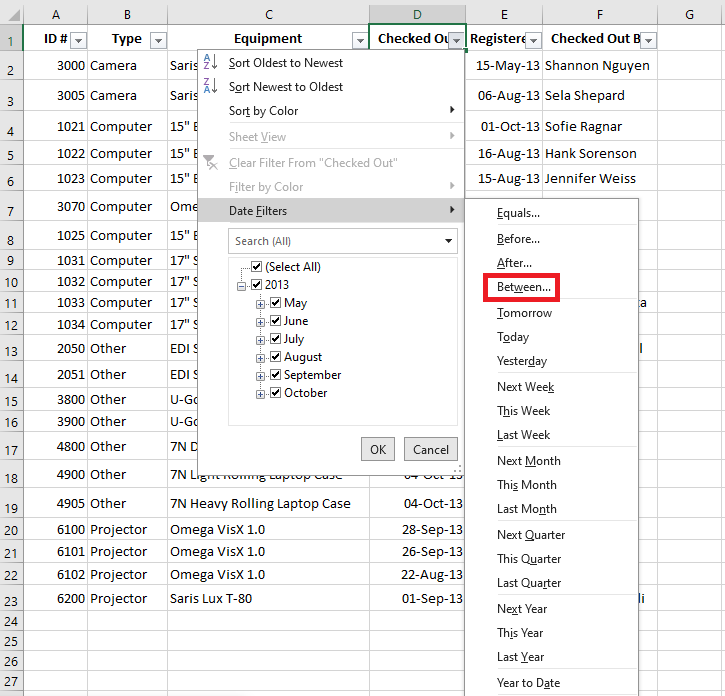
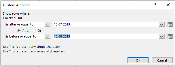
To filter equipment retrieved between July 15 and August 15:
-
Click the dropdown arrow in the Date column (D).
-
Hover over Date Filters, and choose Between…
-
Enter 15-07-2013 and 15-08-2013 (or in your local format), then click OK.
-
The spreadsheet will display only items retrieved within this date range.
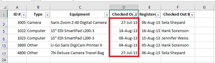
These filtering techniques are powerful tools for managing large datasets efficiently in Excel. Whether you’re dealing with text, numbers, or dates, filters allow you to quickly extract meaningful insights from your data.
-
Inserting Total Rows in Excel Tables
Adding a Total Row to Your Excel Table
Once your dataset has been converted into an Excel Table, adding a Total Row becomes a simple and powerful feature that enhances your data analysis. There are two main methods to add a Total Row:
Method 1: Using the Ribbon
-
Click anywhere inside your Excel Table.
-
Go to the Table Design tab on the Ribbon (also called Design in some versions).
-
In the Table Style Options group, check the box labeled Total Row.
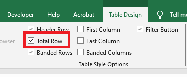
You will now see a new row added at the bottom of your table, displaying the total for the last column by default.
Method 2: Using the Right-Click Menu
-
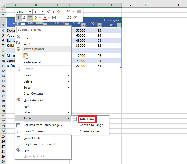
Right-click any cell within your Excel Table.
-
Hover over Table in the context menu.
-
Click Total Row from the submenu.
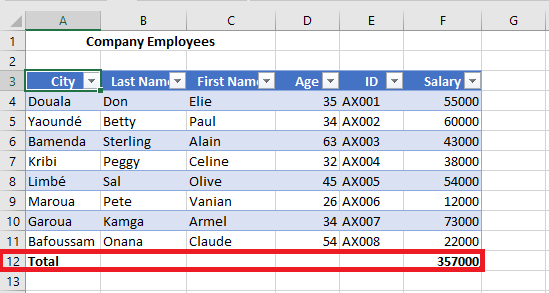
Whichever method you use, Excel will insert a Total Row at the bottom of the table. By default, it will apply the SUM function to the last column, but this can easily be changed.
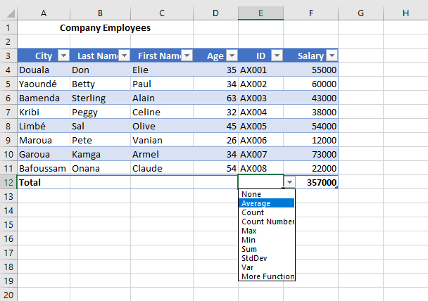
Once the Total Row appears, you can customize each cell in that row. Simply click any cell in the Total Row and a drop-down arrow will appear. This drop-down gives you a variety of aggregation functions to choose from.
Using Other Aggregation Functions in the Total Row
The Total Row is not limited to just sums. It can also display other summary statistics such as:
-
Average
-
Minimum (Min)
-
Maximum (Max)
-
Count
-
Standard Deviation
-
Or even a custom formula of your choice.
For example, if you want to display the average age from an « Age » column:
-
Click the cell in the Total Row that corresponds to the Age column.
-
Click the drop-down arrow that appears.
-
Choose Average from the list.
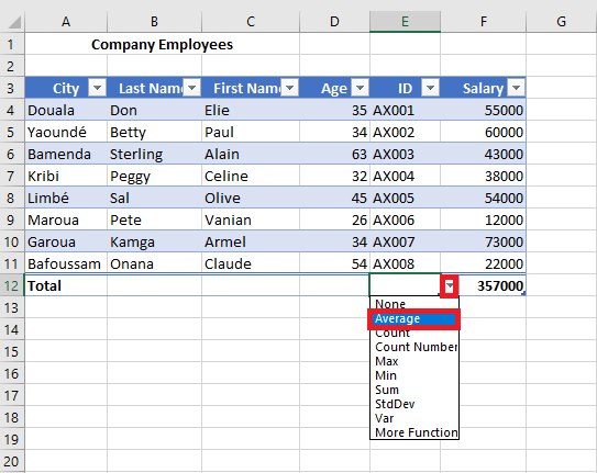
The cell will now display the average of all values in the Age column.
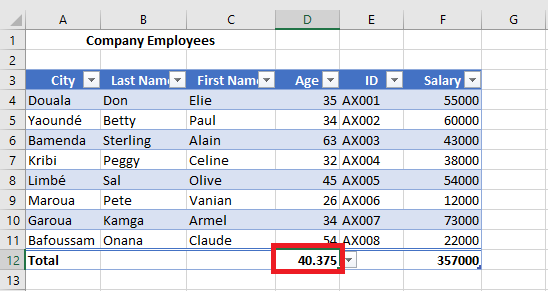
Most of these calculations use the
SUBTOTALfunction, which you can observe in the formula bar. The advantage of usingSUBTOTALis that it automatically adjusts when you filter your table — it calculates only the visible (filtered) values.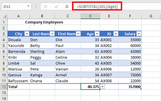
If the predefined list does not offer the function you need, you can insert a different one manually:
-
Click the cell in the Total Row for the desired column.
-
Click the drop-down arrow.
-
Select More Functions at the bottom of the list.
- The Insert Function dialog box will appear, allowing you to choose from any Excel function.
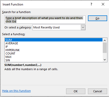
This flexibility allows you to perform customized summaries directly within your table, making the Total Row a valuable tool for quick insights.
-
How to Remove Table Formatting in Excel
By default, Excel tables come with a wide range of built-in features, including predefined table styles that enhance readability and presentation. However, in certain scenarios, you may want to remove the table’s formatting while preserving its structure and functionality.
Remove Table Style Formatting Only
If your goal is to remove the default table style but keep the benefits of a functional Excel table (such as automatic expansion, structured references, and filter buttons), follow these steps:
-
Click on any cell within the table.
-
Go to the Table Design tab (or Design tab under older versions).
-
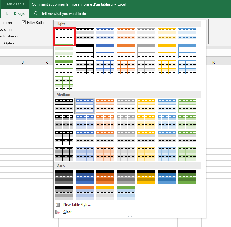
In the Table Styles group, click the very first style under the Light category, labeled None.
- Alternatively, click the dropdown arrow (the « More » button) in the Table Styles gallery, then click Clear at the bottom of the list.
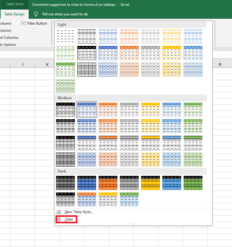
This will strip away the applied style, but your data will remain in a fully functional Excel table — just without the visual enhancements.
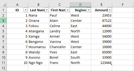
BEFORE
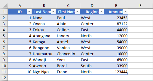
AFTER
-
These options only remove the built-in style formatting. Any custom formatting (such as fonts, colors, borders, etc.) that was manually applied will remain.
-
This method is especially useful when you want to leverage Excel table features but retain your existing cell formatting. Simply convert your data to a table, then clear the style to preserve your custom appearance.
-
To apply a new look, you can always choose another style from the table style gallery.
Clear All Formatting from a Table
If some formatting remains after clearing the table style — such as custom fills, fonts, or borders — it means that manual formatting was applied. To completely remove all formatting (both predefined and custom), do the following:
-
Click on any cell in the table.
-
Press Ctrl + A twice to select the entire table, including headers.
-
Navigate to the Home tab.
-
In the Editing group, click Clear → Clear Formats.

This action will remove all forms of formatting, including:
-
Table styles
-
Manually applied cell formatting
-
Number formats
-
Text alignment
-
Font colors and fills
Caution: This method will reset all formatting. Ensure you’re okay with losing number formats, alignments, and any other styling before proceeding.
BEFORE
AFTER
-
How to Customize and Apply Table Styles in Excel
Creating and managing custom table styles in Excel allows you to define consistent formatting that aligns with your personal or organizational preferences. Follow the detailed steps below to create, edit, apply, or remove a custom table style.
Creating a Custom Table Style
-
Navigate to the Home tab on the Ribbon and click Format as Table.
-
At the bottom of the style gallery, click New Table Style to open the customization window.

-
In the New Table Quick Style dialog box, you can assign a custom name to your new style. For this example, we will retain the default name.
-
From the Table Element list, select the component you wish to format first — for instance, Header Row.
-
Click the Format button to open the cell formatting dialog.

-
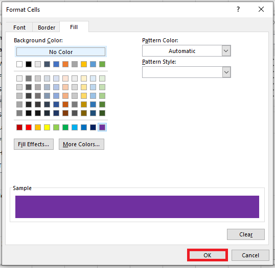
In the Format Cells window, apply the desired formatting options. For example, you can set a specific background color, font style, or border for the header row.
-
Once you’re done with the formatting for that element, click OK to return to the style editor.
-
Repeat the process for other elements in the Table Element list, such as banded rows, total row, or first/last column.
-
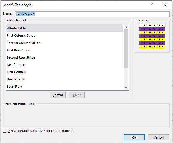
As you make changes, a Preview box shows how your table will look with the applied formatting.
- Optionally, you can adjust the stripe size for banded rows or columns. This determines how many rows or columns each stripe covers.

-
At the bottom, you’ll find a checkbox labeled Set as default table style for this document. Select this if you want all new tables in this workbook to use your custom style by default.
-
When finished, click OK to save the new style.
Your custom table style is now created and available for use in the current workbook.
Applying a Custom Table Style
-
Select any cell within the range you wish to convert into a table.
-
Click Format as Table in the Home tab toolbar.
-
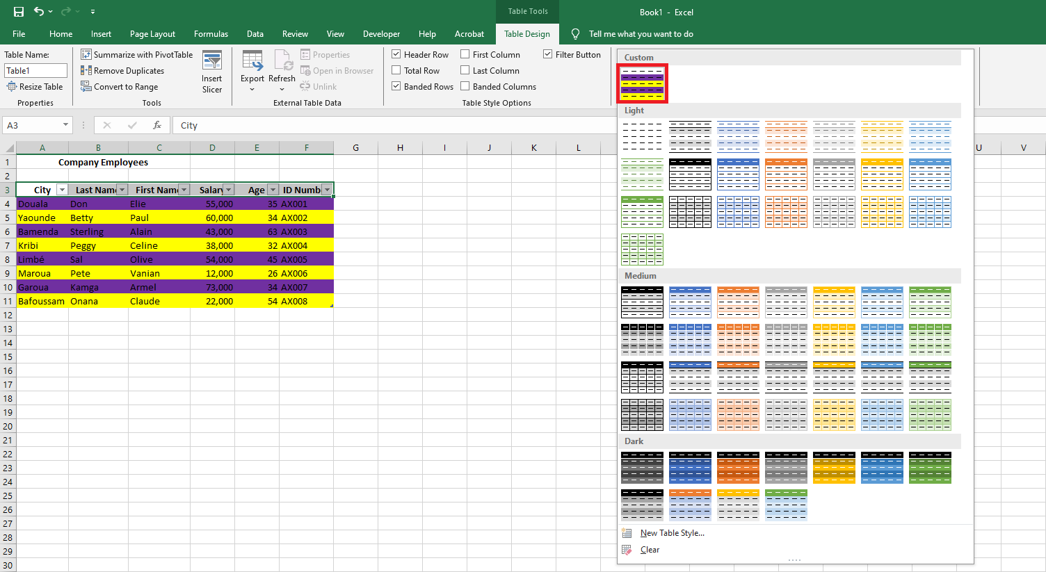
Scroll through the style gallery to locate your newly created style.
-
Hover over the style to preview how it would look on your table.
-
Click on the style to apply it.
Note: Custom table styles are workbook-specific. They will not be available in other Excel files unless redefined.
Modifying a Custom Table Style
-
Go to the Format as Table menu in the Ribbon.
-
Right-click on the custom style you wish to change.
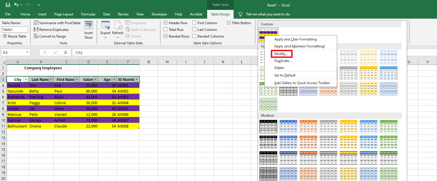
- From the context menu, select Modify. This reopens the style editor where you can change the formatting settings.
- Alternatively, if you want to create a slightly different version while keeping the original intact, choose Duplicate instead.
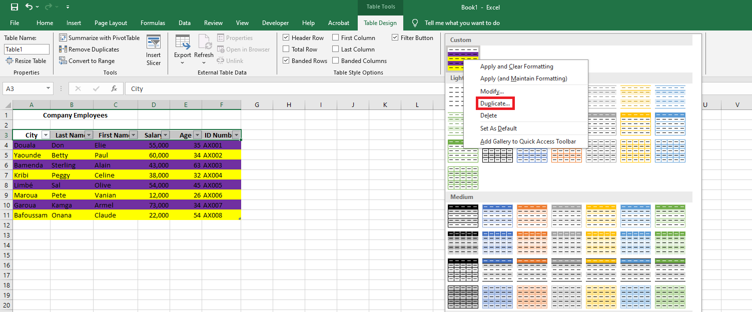
- Excel will append “2” to the name of the duplicated style, which you can rename as needed.

-
Click OK once you’ve finalized the changes. Now, both the original and duplicated styles will appear in the gallery.

Deleting a Custom Table Style
If a custom style is no longer needed and hasn’t been applied to any tables, you can remove it to free up memory.
-
Open the Format as Table menu.
-
Right-click the style you want to remove.
- Select Delete from the context menu.

-
Confirm the deletion by clicking OK when prompted.
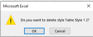
If any tables currently use the deleted style, Excel will revert them to the default formatting.
-