Votre panier est actuellement vide !
Catégorie : Excel VBA Course
Example: Moving Cells in Excel VBA
In the very first macro presented in this book, a recorded macro was used to move the contents of one cell to another:
Sub Macro1()
    Range("A1").Select
    Selection.Cut
    Range("C1").Select
    ActiveSheet.Paste
End Sub
Disadvantages of this approach:
- Multiple steps are required, increasing the chance of errors.
- It is unclear which workbook and worksheet the move operation applies to.
- The process runs more slowly.
Using direct referencing, you can perform this task more clearly and efficiently:
Sub MoveCells()
    ThisWorkbook.Worksheets("Sheet1").Range("A7:A9").Cut _
        Destination:=ThisWorkbook.Worksheets("Sheet1").Range("B7")
End Sub
This method clearly specifies the source and destination ranges within the same workbook and worksheet. It avoids unnecessary selection and pasting steps, resulting in faster and more reliable code.
The Application.InputBox Method In Excel VBA
The Application.InputBox() method provides better input control and overall more options than the basic InputBox(). Its return value depends on the type specified. You can choose the input type to be a number, formula, cell reference, text, or Boolean value. If the user clicks Cancel, the method returns False, which you can use to control the flow of your program.
Like the simple input box, you can specify a default value and a title. The input type is set using the last parameter. Therefore, the examples below use named parameters for clarity.
Entering a Number
Here is an example where a number is requested (Type 1):
Sub EnterNumber()
    ThisWorkbook.Worksheets("Sheet1").Activate
    Range("A1").Value = Application.InputBox(Prompt:="Number:", Type:=1)
End Sub
Explanation:
You can run the EnterNumber() procedure through the Macro dialog box, accessible via the Excel ribbon under the View tab → Macros → View Macros. Alternatively, you can create a button on the worksheet and link it to this procedure.If the user inputs a valid number, it is placed in cell A1. Valid examples include « 5.7 », « 5e2 » (which equals 5 × 10² = 500), or « 0.57 ». Invalid examples are « 5a7 » or « a57 ». Note that entering « 5.7 » might be interpreted as the date July 5 of the current year depending on regional settings.
If the user inputs an invalid number, a warning message appears, and the input box remains open until a valid number is entered, as shown in Figure 8.5.
Entering a Formula
An example to input a formula (Type 0):
Sub EnterFormula()
    ThisWorkbook.Worksheets("Sheet1").Activate
    Range("A1").Value = Application.InputBox(Prompt:="Formula:", Type:=0)
End Sub
Explanation:
Run EnterFormula() via the Macro dialog or a button. The user can enter formulas including cell references, which may also cover non-contiguous ranges.Typing =SUM($A$10:$A$12) will insert this formula into cell A1, showing the calculated result. Pay attention to the use of absolute references with dollar signs.
If the user starts typing =SUM(, they can select the cells using the mouse or arrow keys before closing the parenthesis.
Entering an invalid formula results in an error message.
Entering a Cell Range
An example for entering a cell range (Type 8):
Sub EnterRange()
    Dim rng As Range
    ThisWorkbook.Worksheets("Sheet1").Activate
    Set rng = Application.InputBox(Prompt:="Cell range:", Type:=8)
    rng.Borders.LineStyle = xlContinuous
    Set rng = Nothing
End Sub
Explanation:
Run EnterRange() through the Macro dialog or a button. First, an object variable for a Range object is declared.The user can input ranges by typing or selecting with the mouse. Non-contiguous ranges are also supported. Remember to use absolute references with dollar signs for non-contiguous areas.
The selected range is returned and stored in the object variable, allowing further actions such as formatting or calculations.
Additional Notes
Besides the types described above—
- 1 for numbers,
- 0 for formulas, and
- 8 for ranges,
there are other type codes available, for example:
- 2 for text input, and
- 4 for Boolean values.
The InputBox Function In Excel VBA
The return value of the InputBox() function is always a string. The input field can be pre-filled with a default value, which helps guide the user or speeds up data entry. To make it clear what the user should enter, both a prompt message and a dialog title can be displayed.
In the following example, the user is asked successively to enter a text, a number, and a date:
Sub SimpleInput()
    ThisWorkbook.Worksheets("Sheet1").Activate
    Dim userInput As String
    Range("A1").Value = InputBox("Please enter text", "Text", "Moyo")
    userInput = InputBox("Please enter a number", "Number", "2")
    If userInput = "" Then
        Range("A2").Value = ""
    Else
        Range("A2").Value = CDbl(userInput)
    End If
    userInput = InputBox("Please enter a date (D.M.YY)", "Date", "04.06.25")
    If userInput = "" Then
        Range("A3").Value = ""
    Else
        Range("A3").Value = CDate(userInput)
    End If
End Sub
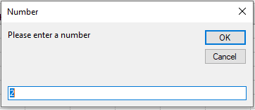
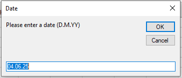
Figure illustrates the result after the second call to the InputBox() function.
Explanation:
Each time, a dialog box appears showing the prompt text, a title, and a default value.- If the user clicks OK, the contents of the input field are returned as a string.
- If the user clicks Cancel, an empty string is returned.
When the user is expected to enter a number, you should check the returned string and then convert it to a Double using the CDbl() function. The user can use the familiar decimal comma to separate fractional parts, depending on regional settings.
Similarly, when the user is expected to enter a date, you should check the returned string and convert it to a date value using the CDate() function.
Reading Formulas In Excel VBA
The worksheet function IsFormula() has been available since Excel 2013. It determines whether a cell contains a formula. If this is the case, the formula of the cell can be retrieved and displayed using the various versions of the Formula property.
Below is an example where the range from A10 to A14 is checked for formulas. The formulas in cells A13 and A14 are displayed in all four property versions.
Sub FormulaVersions()
    ThisWorkbook.Worksheets("Sheet1").Activate
    Range("A13").Formula = "=A10 + A11 + A12"
    Range("A14").Formula = "=SUM(A10:A12)"
    Range("A15").FormulaLocal = "=A10 + A11 + A12"
    Range("A16").FormulaLocal = "=SUM(A10:A12)"
    Range("A17").FormulaR1C1 = "=R[-7]C + R[-6]C + R[-5]C"
    Range("A18").FormulaR1C1 = "=SUM(R[-8]C:R[-6]C)"
    Range("A19").FormulaR1C1Local = "=R[-9]C + R[-8]C + R[-7]C"
    Range("A20").FormulaR1C1Local = "=SUM(R[-10]C:R[-8]C)"
End Sub

Sub DisplayFormulas()
    Dim i As Integer
    ThisWorkbook.Worksheets("Sheet1").Activate
    For i = 10 To 14
        If WorksheetFunction.IsFormula(Cells(i, 1)) Then
            MsgBox Cells(i, 1).Address & vbCrLf & _
                   Cells(i, 1).Formula & vbCrLf & _
                   Cells(i, 1).FormulaLocal & vbCrLf & _
                   Cells(i, 1).FormulaR1C1 & vbCrLf & _
                   Cells(i, 1).FormulaR1C1Local & vbCrLf
        End If
    Next i
End Sub
Figures:
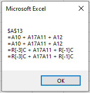
Addition formula in cell A13 – shown in four versions
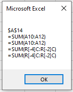
Sum formula in cell A14 – shown in four versions
Notes:
For versions of Excel prior to 2013, the loop index i should run only from 13 to 14 because IsFormula() is not available. Additionally, the condition using IsFormula() should be omitted.Sometimes you will see the notation Application.WorksheetFunction.IsFormula() used as well. However, the top-level object name Application can usually be omitted.
Formulas In Excel VBA
This section explains the differences and similarities among the cell properties Formula, FormulaLocal, FormulaR1C1, and FormulaR1C1Local using an example with various assignments:
Sub FormulaVersions()
    ThisWorkbook.Worksheets("Sheet1").Activate
    Range("A13").Formula = "=A10 + A11 + A12"
    Range("A14").Formula = "=SUM(A10:A12)"
    Range("A15").FormulaLocal = "=A10 + A11 + A12"
    Range("A16").FormulaLocal = "=SUM(A10:A12)"
    Range("A17").FormulaR1C1 = "=R[-7]C + R[-6]C + R[-5]C"
    Range("A18").FormulaR1C1 = "=SUM(R[-8]C:R[-6]C)"
    Range("A19").FormulaR1C1Local = "=R[-9]C + R[-8]C + R[-7]C"
    Range("A20").FormulaR1C1Local = "=SUM(R[-10]C:R[-8]C)"
End Sub
Explanation:
Each line calculates the sum of the numbers in the three cells from A10 to A12, but using different ways to assign the formula.- The Formula property expects the formula to be assigned in English notation. Inside the string, either a calculation expression using the plus operator (+) or the worksheet function SUM() can be used. The spaces inside the formula string are added only for readability and can be omitted without affecting functionality.
- The FormulaLocal property expects the formula to be assigned in the local language notation—in this case, German. The calculation expression with the plus operator (+) remains the same as in English. However, the worksheet function must be written as SUMME() instead of SUM().
- The FormulaR1C1 property expects the formula in English notation but uses relative cell references based on the R1C1 reference style. Here, R stands for « Row » and C for « Column ». Relative positions are specified inside square brackets. For example:
- RC refers to the current cell.
- R[-1]C refers to the cell one row above the current cell.
- RC[-1] refers to the cell one column to the left.
- R[-1]C[-1] refers to the cell diagonally up-left from the current cell.
- The FormulaR1C1Local property expects the formula in the local language notation and also uses relative cell references, but with a different syntax. Here, Z stands for « Zeile » (row) and S stands for « Spalte » (column). Relative positions are specified inside parentheses (round brackets), not square brackets. The examples above for R and C apply analogously to Z and S notation:
- ZS is the current cell.
- Z(-1)S is the cell one row above.
- ZS(-1) is the cell one column to the left.
- Z(-1)S(-1) is the cell diagonally up-left.
Cropping Pictures In Excel VBA
The following program inserts the picture from the previous example multiple times at a reduced size of 100 × 75 points. Different parts of the images are cropped. The crop values must relate to the original image size of 288 × 216 points. For example, to display only the left or right half of the image, a crop value of 144 points is required.
Sub CropPictures()
    Dim Sh(1 To 6) As Shape
    Dim X As Shape
    Dim FilePath As String
    Dim i As Integer
    ThisWorkbook.Worksheets("Sheet10").Activate
    FilePath = ThisWorkbook.Path & "C:\Users\POPOLY\Desktop\fleur.jpeg"
    ' Delete all existing shapes
    For Each X In ActiveSheet.Shapes
        X.Delete
    Next X
    ' Insert images and crop different parts
    Set Sh(1) = ActiveSheet.Shapes.AddPicture(FilePath, msoFalse, msoTrue, 10, 10, 100, 75)
    Set Sh(2) = ActiveSheet.Shapes.AddPicture(FilePath, msoFalse, msoTrue, 10, 95, 100, 75)
    Sh(2).PictureFormat.CropLeft = 144 ' Crop left half
    Set Sh(3) = ActiveSheet.Shapes.AddPicture(FilePath, msoFalse, msoTrue, 10, 180, 100, 75)
    Sh(3).PictureFormat.CropRight = 144 ' Crop right half
    Set Sh(4) = ActiveSheet.Shapes.AddPicture(FilePath, msoFalse, msoTrue, 120, 10, 100, 75)
    Sh(4).PictureFormat.CropTop = 108 ' Crop top half
    Set Sh(5) = ActiveSheet.Shapes.AddPicture(FilePath, msoFalse, msoTrue, 230, 10, 100, 75)
    Sh(5).PictureFormat.CropBottom = 108 ' Crop bottom half
    Set Sh(6) = ActiveSheet.Shapes.AddPicture(FilePath, msoFalse, msoTrue, 230, 180, 100, 75)
    Sh(6).PictureFormat.CropRight = 144 ' Crop right half
    Sh(6).PictureFormat.CropBottom = 108 ' Crop bottom half
    ' Output properties for overview
    Cells(1, 8).Value = "Number"
    Cells(1, 9).Value = "Left"
    Cells(1, 10).Value = "Top"
    Cells(1, 11).Value = "Width"
    Cells(1, 12).Value = "Height"
    For i = 1 To 6
        Cells(i + 1, 8).Value = i
        Cells(i + 1, 9).Value = Sh(i).Left
        Cells(i + 1, 10).Value = Sh(i).Top
        Cells(i + 1, 11).Value = Sh(i).Width
        Cells(i + 1, 12).Value = Sh(i).Height
        Set Sh(i) = Nothing
    Next i
End Sub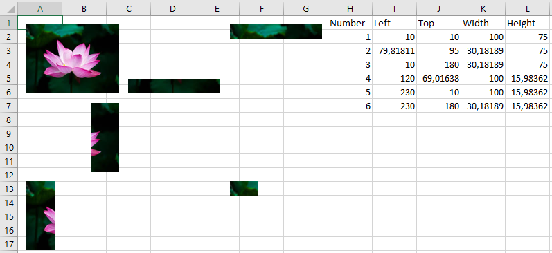
Explanation:
References to the six picture objects are stored in an array.The file path is assigned, and all existing shapes on the worksheet are deleted.
The first picture object is inserted at the top-left and is not cropped. It serves as a reference for comparison with the other five pictures.
The PictureFormat property of a Shape object allows manipulation of the picture, including cropping.
The second picture is inserted below the first, with the left half cropped (CropLeft = 144).
The third picture is inserted below the second, cropping the right half (CropRight = 144).
The fourth picture is placed to the right of the first, cropping the top half (CropTop = 108).
The fifth picture is placed right of the fourth, cropping the bottom half (CropBottom = 108).
The sixth picture is placed at the bottom right, cropping both the right half and bottom half (CropRight = 144 and CropBottom = 108), leaving only the upper-left quarter visible.
Inserting a Picture In Excel VBA
The following program inserts a picture into the worksheet:
Sub InsertPicture()
    Dim Sh As Shape
    ThisWorkbook.Worksheets("Sheet10").Activate
    ' Delete all existing shapes on the sheet
    For Each Sh In ActiveSheet.Shapes
        Sh.Delete
    Next Sh
    ' Add picture from file
    Set Sh = ActiveSheet.Shapes.AddPicture( _
        ThisWorkbook.Path & "C:\Users\POPOLY\Desktop\fleur.jpeg", _
        msoFalse, msoTrue, 10, 10, -1, -1)
    ' Display position and size of the inserted picture
    MsgBox Sh.Left & "/" & Sh.Top
    MsgBox Sh.Width & "/" & Sh.Height
End Sub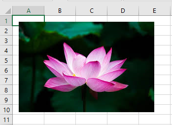
Explanation:
The variable Sh is used as a reference to the picture object.First, all existing shapes on the worksheet are deleted.
The method AddPicture() of the Shapes collection adds a picture object from an image file.
The first parameter is the file path and name.
The second parameter, set to msoFalse, specifies that the picture is embedded as a copy inside the Excel file. If set to msoTrue, the picture would be linked to the external image file, so changes to the file would update the Excel image.
The third parameter further controls linking behavior. Since the picture is embedded here, this is set to msoTrue.
The fourth and fifth parameters specify the distance in points from the left and top edges of the worksheet to the top-left corner of the image.
The last two parameters set the width and height of the image in points. Here, both are set to -1, which causes the picture to be displayed at its original size. For example, an image sized 400 × 300 pixels corresponds approximately to 288 × 216 points.
The return value of AddPicture() is a reference to the Shape object, through which you can read the position properties (Left and Top) and size properties (Width and Height) in points.
SmartArt In Excel VBA
SmartArt graphics allow you to quickly and clearly represent relationships, processes, or hierarchies.It was created via the menu: INSERT • SMARTART • LIST • SIMPLE BLOCK LIST. Afterwards, the text was modified through the text pane, and the graphic was repositioned.
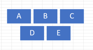
In VBA, a SmartArt graphic is treated as a group of shapes. However, the properties of these shapes can only be read, not modified.
The following program outputs the positions of the individual blocks:
Sub ReadSmartArtPositions()
    Dim i As Integer
    Dim s As String
    Dim Sh As Shape
    ' Select the first SmartArt object
    Set Sh = ThisWorkbook.Worksheets("Sheet9").Shapes(1)
    ' Collect the Top and Left positions of all group items
    For i = 1 To Sh.GroupItems.Count
        s = s & Int(Sh.GroupItems(i).Top) & _
            " " & Int(Sh.GroupItems(i).Left) & vbCrLf
    Next i
    MsgBox s
    Set Sh = Nothing
End Sub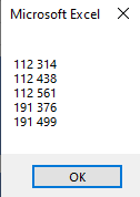
Explanation:
The GroupItems collection contains all elements within the SmartArt group.Each individual element of the group can be accessed by its index.
The Top and Left properties of each block are gathered and displayed in a message box, as illustrated in Figure.
All Colors In Excel VBA
The following program provides an overview of all available colors for sparklines, both for bars and lines:
Sub DisplaySparklineColors()
    Dim i As Integer
    ThisWorkbook.Worksheets("Sheet8").Activate
    For i = 1 To 11
        Cells(i + 13, 1).SparklineGroups.Add _
            xlSparkColumn, "A1:A10"
        Cells(i + 13, 1).SparklineGroups.Item(1). _
            SeriesColor.ThemeColor = i
    Next i
    ' Set background color for better visibility of white bars
    Cells(14, 1).Interior.Color = vbBlack
End Sub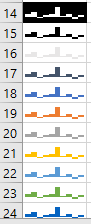
Explanation:
The colors are numbered from 1 to 11.For clearer visibility, the cell containing the white bars is given a black background.
Formatting a Sparkline In Excel VBA
Certain values in a sparkline can be highlighted, and colors can be customized. Here is an example:
Sub FormatLineSparkline()
    ThisWorkbook.Worksheets("Sheet8").Activate
    With Range("A11").SparklineGroups
        .Add xlSparkLine, "A1:A10"
        .Item(1).SeriesColor.ThemeColor = 2
        .Item(1).Points.Markers.Visible = True
        .Item(1).Points.Markers.Color.ThemeColor = 10
        .Item(1).Points.Negative.Visible = True
        .Item(1).Points.Negative.Color.ThemeColor = 9
    End With
End Sub
Explanation:
First, the color of the sparkline is changed via the ThemeColor sub-property of the SeriesColor property for the first element in the SparklineGroups collection. The possible theme colors will be demonstrated in a subsequent example.Data points are given visible markers with a specific color. This is controlled by properties of the Markers object within the Points collection: first, the Visible property is set to True, then the ThemeColor sub-property of the Color property is set to specify the marker color.
Negative points are also highlighted and colored using the Negative property, with visibility enabled and a theme color assigned.