Catégorie : Excel VBA Course

Finally, here is a win-loss indicator represented by bars that distinguish positive and negative values:

Sub CreateWinLossSparkline()
    ThisWorkbook.Worksheets("Sheet8").Activate
    Range("A11").SparklineGroups.Add _
        xlSparkColumnStacked100, "A1:A10"
End Sub

Explanation:
The element xlSparkColumnStacked100 from the xlSparkType enumeration creates a sparkline that visually differentiates between positive and negative values using stacked columns.

A sparkline of the column type is created in a similar manner:

Sub CreateColumnSparkline()
    ThisWorkbook.Worksheets("Sheet8").Activate
    Range("A11").SparklineGroups.Add xlSparkColumn, "A1:A10"
End Sub

Explanation:
This time, the element xlSparkColumn from the xlSparkType enumeration is used, which generates a series of vertical bars representing the data.

The following program creates a sparkline of the line type:

Sub CreateLineSparkline()
    ThisWorkbook.Worksheets("Sheet8").Activate
    Range("A11").SparklineGroups.Add xlSparkLine, "A1:A10"
End Sub

Explanation:
The Add() method of the SparklineGroups collection creates a SparklineGroup object in the target cell (here, cell A11).

The first parameter, Type, is set to xlSparkLine from the xlSparkType enumeration, specifying a line sparkline.

The second parameter is a string representing the source data range for the sparkline values (here, cells A1 through A10).

Instead of using data bars or color scales, the relative sizes of a series of numbers can also be visually represented using different symbols, as shown in the following program:

Sub IconSetExample()
    Dim Rg As Range
    ThisWorkbook.Worksheets("Sheet6").Activate
    Set Rg = Range("A2:A11")
    ' Remove existing conditional formats
    Rg.FormatConditions.Delete
    ' Add icon set conditional formatting
    Rg.FormatConditions.AddIconSetCondition
    ' Modify icon set settings
    With Rg.FormatConditions(1)
        .IconSet = ActiveWorkbook.IconSets(1)
        .IconCriteria(2).Value = 45
        .IconCriteria(3).Value = 90
    End With
    Set Rg = Nothing
End Sub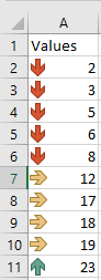

Explanation:
The AddIconSetCondition() method creates an object of the class IconSetCondition, which is a conditional formatting rule using an icon set.

The type of icon set can be changed by assigning an element from the IconSets collection of the active workbook to the IconSet property of the conditional format.

Icon sets can contain three, four, or five different icons. In this example, a three-icon set is used.

New threshold values are set for the second and third icons by modifying the Value property of the second and third elements in the IconCriteria collection.

For example, if a cell contains a value at least 45% of the maximum value in the range, the second icon is displayed; for 90% or more, the third icon is shown. By default, the thresholds are 34% and 67%.

Excel 2007 already includes 17 different icon sets, and Excel 2010 added three more. The following program displays all 20 icon sets neatly:

Sub DisplayAllIconSets()
    Dim Rg As Range
    Dim i As Integer
    ThisWorkbook.Worksheets("Sheet7").Activate
    For i = 1 To 20
        Range("A2:A11").Copy Cells(2, i)
        Cells(1, i).Value = "S " & i
        Set Rg = Range(Cells(2, i), Cells(11, i))
        Rg.FormatConditions.Delete
        Rg.FormatConditions.AddIconSetCondition
        Rg.FormatConditions(1).IconSet = ActiveWorkbook.IconSets(i)
    Next i
    Set Rg = Nothing
End Sub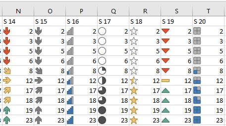

Explanation:
The values in the first column are copied into the subsequent columns.

For each column, a range of ten cells is selected for conditional formatting.

An icon set conditional format is created for each range, with the icon set type assigned from the 20 available options.

The following example demonstrates a three-color scale:

Sub ThreeColorScale()
    Dim Rg As Range
    ThisWorkbook.Worksheets("Sheet6").Activate
    Set Rg = Range("A2:A11")
    ' Remove any existing conditional formats
    Rg.FormatConditions.Delete
    ' Add a three-color scale conditional formatting
    Rg.FormatConditions.AddColorScale 3
    ' Modify the three-color scale settings
    With Rg.FormatConditions(1)
        .ColorScaleCriteria(1).Type = xlConditionValueLowestValue
        .ColorScaleCriteria(1).FormatColor.Color = vbGreen
        .ColorScaleCriteria(2).Type = xlConditionValuePercentile
        .ColorScaleCriteria(2).FormatColor.Color = vbYellow
        .ColorScaleCriteria(3).Type = xlConditionValueHighestValue
        .ColorScaleCriteria(3).FormatColor.Color = vbRed
    End With
    Set Rg = Nothing
End Sub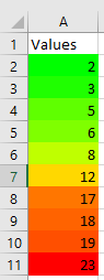

Explanation of Differences from Two-Color Scale:
The method AddColorScale() is called with the parameter value 3 to specify a three-color scale.

When modifying the scale, the middle color corresponds to the percentile value (xlConditionValuePercentile), which represents a statistical intermediate value.

This middle color is set to yellow, while the lowest and highest values are colored green and red respectively.

It is possible to format a range of cells using either a two-color or three-color scale. Here is an example using a two-color scale:

Sub TwoColorScale()
    Dim Rg As Range
    ThisWorkbook.Worksheets("Sheet6").Activate
    Set Rg = Range("A2:A11")
    ' Remove any existing conditional formats
    Rg.FormatConditions.Delete
    ' Add a two-color scale conditional formatting
    Rg.FormatConditions.AddColorScale 2
    ' Modify the two-color scale settings
    With Rg.FormatConditions(1)
        .ColorScaleCriteria(1).Type = xlConditionValueLowestValue
        .ColorScaleCriteria(1).FormatColor.Color = vbYellow
        .ColorScaleCriteria(2).Type = xlConditionValueHighestValue
        .ColorScaleCriteria(2).FormatColor.Color = vbRed
    End With
    Set Rg = Nothing
End Sub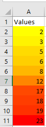

Explanation:
First, any existing conditional formats in the specified range are deleted.

The method AddColorScale() creates a ColorScale object, which is a conditional formatting rule using a color gradient. The first parameter (ColorScaleType) determines whether the scale is two-colored or three-colored.

Additional formatting criteria can be set on a ColorScale object via its ColorScaleCriteria collection.

For the first criterion, the lowest value in the range is assigned the color yellow. This is done by setting the Type property to xlConditionValueLowestValue (from the xlConditionValueTypes enumeration) and assigning the desired color to the FormatColor.Color property.

For the second criterion, the highest value is assigned the color red, using the xlConditionValueHighestValue enumeration.

The following program illustrates the relative sizes of a series of numbers using data bars:

Sub CreateDataBars()
    Dim Rg As Range
    ThisWorkbook.Worksheets("Sheet6").Activate
    Set Rg = Range("A2:A11")
    ' Remove any existing conditional formats
    Rg.FormatConditions.Delete
    ' Add data bars conditional formatting
    Rg.FormatConditions.AddDatabar
    ' Modify the data bar color
    Rg.FormatConditions(1).BarColor.Color = vbRed
    Set Rg = Nothing
End Sub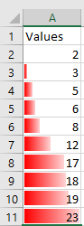

Explanation:
Conditional formatting rules applied to a cell or a range are stored in the FormatConditions collection.

The Delete() method removes any existing conditional formats in the specified range.

The AddDatabar() method adds a data bar conditional formatting rule, which creates a bar inside each cell reflecting the relative value within the range.

Since this is the first conditional format applied, it is accessed by the index 1. Additional conditional formats could later be added and accessed by higher indices.

The color of the data bar is modified through the BarColor.Color property.

Figure shows the resulting data bars visualization.

WordArt allows you to create decorative text effects, such as shadowed or mirrored text. Using the method AddTextEffect(), the following example displays an overview of the 30 different predefined effect types available up to Excel 2010. Since Excel 2013, 20 additional effect types have been introduced. Each resulting object is of the class Shape.

Code:

Sub DisplayAllWordArt()
    Dim Sh As Shape
    Dim i As Integer, lf As Integer, tp As Integer
    ' Select the worksheet
    ThisWorkbook.Worksheets("Sheet5").Activate
    ' Hide gridlines for clearer display
    ActiveWindow.DisplayGridlines = False
    ' Delete all existing shapes
    For Each Sh In ActiveSheet.Shapes
        Sh.Delete
    Next Sh
    ' Initial position values
    lf = 5
    tp = 5
    ' Create all available WordArt presets
    For i = 0 To 49
        Set Sh = ActiveSheet.Shapes.AddTextEffect( _
            i, CStr(i), "Arial", 48, False, False, lf, tp)
        Sh.TextFrame.Characters.Font.Color = RGB(255, 0, 0)
        ' Calculate position for next WordArt object
        lf = lf + 70
        If i Mod 6 = 5 Then
            lf = 10
            tp = tp + 70
        End If
    Next i
    Set Sh = Nothing
End Sub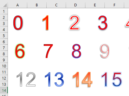

Explanation:
As in the previous program, gridlines on the worksheet are hidden, and any existing shapes are deleted.

After setting the initial position, the loop calls the method AddTextEffect(), which has eight mandatory parameters:

• Type of predefined text effect
• Text to display
• Font name
• Font size
• Bold: True/False
• Italic: True/False
• Left position
• Top position

The font color of the text inside the shape’s text frame is set to red.

At the end of each loop iteration, the position for the next WordArt object is calculated.

The effect can be further customized using the parameters.

Figure shows a small excerpt displaying WordArt types.

For better clarity, this section demonstrates all the different AutoShapes using the following VBA program:

Sub DisplayAllShapes()
    Dim Sh As Shape
    Dim i As Integer, lf As Integer, tp As Integer
    ' Select the worksheet
    ThisWorkbook.Worksheets("Sheet4").Activate
    ' Hide gridlines for clearer display
    ActiveWindow.DisplayGridlines = False
    ' Delete all existing shapes
    For Each Sh In ActiveSheet.Shapes
        Sh.Delete
    Next Sh
    ' Initial position values
    lf = 5
    tp = 5
    ' Create all possible shapes
    For i = 1 To 137
        Set Sh = ActiveSheet.Shapes.AddShape(i, lf, tp, 30, 30)
        ' Format the shape
        With Sh
            .Line.Weight = 1
            .Line.ForeColor.RGB = RGB(0, 0, 0)
            .Fill.ForeColor.RGB = RGB(255, 255, 255)
        End With
        ' Add the shape type number as text inside the shape
        With Sh.TextFrame.Characters
            .Font.Color = vbBlack
            .Font.Size = 7
            .Text = i
        End With
        ' Calculate position for next shape
        lf = lf + 35
        If i Mod 15 = 0 Then
            lf = 5
            tp = tp + 35
        End If
    Next i
    Set Sh = Nothing
End Sub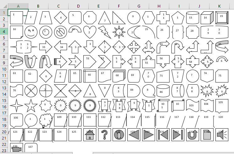

Explanation:
First, gridlines on the worksheet are hidden to improve visibility. Then, any existing shapes on the sheet are deleted.

Initial coordinates for placing the AutoShapes are set.

Within the loop, all 137 different AutoShapes are created using the AddShape() method.

Each shape is sized 30 by 30 points, drawn with a thin black border and a white fill.

Inside each shape, its Type number (the current loop index) is displayed as text.

At the end of each loop iteration, the position for the next shape is calculated, moving horizontally by 35 points and moving down a row every 15 shapes.

The Figure shows a small excerpt of the shapes. Depending on the shape’s design, the type number may only be partially visible, but can always be inferred by the neighboring shapes.

A freeform shape is a path composed of straight or curved line segments connecting vertices (called nodes). If the last node coincides with the first, the freeform is closed, creating an enclosed area.

The method BuildFreeform() creates a FreeformBuilder object starting with the first node. Additional nodes are added with AddNodes(). Finally, ConvertToShape() converts the freeform into a Shape object.

Two examples follow: a closed freeform and an open freeform polyline.

Closed Freeform Example:

Sub ClosedFreeform()
    Dim FB As FreeformBuilder
    Dim Sh As Shape
    ThisWorkbook.Worksheets("Sheet3").Activate
    ' Initialize freeform with first node
    Set FB = ActiveSheet.Shapes.BuildFreeform(msoEditingAuto, 330, 30)
    ' Add curved nodes
    FB.AddNodes msoSegmentCurve, msoEditingAuto, 390, 60
    FB.AddNodes msoSegmentCurve, msoEditingAuto, 390, 120
    FB.AddNodes msoSegmentCurve, msoEditingAuto, 430, 40
    ' Close the freeform by returning to the first node
    FB.AddNodes msoSegmentCurve, msoEditingAuto, 330, 30
    ' Convert freeform to shape and format
    Set Sh = FB.ConvertToShape
    Sh.Line.Weight = 3
    Sh.Fill.ForeColor.RGB = RGB(91, 155, 213)
    Sh.Line.ForeColor.RGB = RGB(65, 113, 156)
    Set Sh = Nothing
    Set FB = Nothing
End Sub

Explanation of Closed Freeform:

The method BuildFreeform() requires three parameters:

• EditingType: defines the editing behavior of the first node and must be a value from the msoEditingType enumeration. The value msoEditingAuto means the editing mode adapts automatically to connected segments, providing a universal setting.
• X1 and Y1: specify the coordinates of the first node.

The AddNodes() method requires at least four parameters:

• SegmentType: defines the type of connection to the new node, from the msoSegmentType enumeration. Possible values include msoSegmentCurve for curved segments and msoSegmentLine for straight lines.
• EditingType: as described above.
• The next two parameters specify the coordinates of the new node when EditingType is set to msoEditingAuto.

The method ConvertToShape() converts the built freeform into a Shape, which can then be manipulated with standard shape properties and methods, such as Line.Weight for line thickness.

Open Freeform Polyline Example:

The node coordinates are taken from the worksheet (see Figure 7.16).

Sub OpenFreeformPolyline()
    Dim FB As FreeformBuilder
    Dim Sh As Shape
    Dim i As Integer
    ThisWorkbook.Worksheets("Sheet3").Activate
    ' Initialize freeform with first node from cells I1 (col 9), J1 (col 10)
    Set FB = ActiveSheet.Shapes.BuildFreeform(msoEditingAuto, Cells(1, 9), Cells(1, 10))
    ' Add line segments for nodes in rows 2 to 10
    For i = 2 To 10
        FB.AddNodes msoSegmentLine, msoEditingAuto, Cells(i, 9), Cells(i, 10)
    Next i
    ' Convert freeform to shape and format
    Set Sh = FB.ConvertToShape
    Sh.Line.Weight = 3
    Sh.Line.ForeColor.RGB = RGB(91, 155, 213)
    Set Sh = Nothing
    Set FB = Nothing
End Sub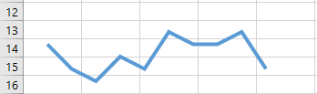

Explanation:
The coordinates for the first node come from the first row of the specified columns, and subsequent nodes come from the rows below. The connection type used here is a straight line (msoSegmentLine).