Votre panier est actuellement vide !
Étiquette : data_analysis
Variance Calculation in Excel
Variance is one of the most useful tools in probability theory and statistics. In science, it describes how far each number in the dataset is from the mean. In practice, it often shows how much something changes. For example, the temperature near the equator has less variance than in other climate zones. In this section, we will analyze various methods to calculate variance in Excel.
What is Variance?
Variance is a measure of the variability of a data set that indicates how spread out the different values are.
Mathematically, variance is defined as the mean of the squared deviations from the mean.
To better understand what you’re actually calculating with variance, let’s consider this simple example:
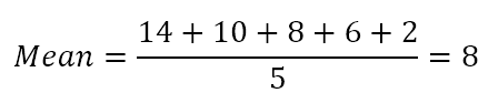
Suppose there are 5 tigers in your local zoo, aged 14, 10, 8, 6, and 2 years.
To find the variance, follow these simple steps:
- Calculate the mean (simple average) of the five numbers:
- Subtract the mean from each number to find the differences.
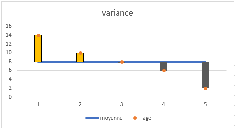
- Square each difference.
- Find the mean of the squared differences.
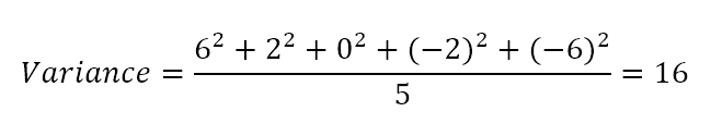
Thus, the variance is 16. But what does this number really mean?
In reality, variance gives you only a very general idea of the dispersion of the dataset. A value of 0 means there is no variability (i.e., all numbers in the dataset are the same). The larger the number, the more spread out the data is.
This example pertains to the population variance (i.e., the 5 tigers represent the entire group of interest). If your data is a selection from a larger population, you would need to calculate the sample variance using a slightly different formula.
How to Calculate Variance in Excel
There are 6 built-in functions in Excel to calculate variance: VAR(), VAR.S(), VARP(), VAR.P(), VARA(), and VARPA().
Your choice of variance formula depends on the following factors:
- The version of Excel you are using.
- Whether you are calculating sample or population variance.
- Whether you want to evaluate or ignore text and logical values.
Here’s an overview of the variance functions available in Excel to help you choose the formula that best suits your needs:
Name Excel Version Data Type Text & Logic Handling VAR 2000 – 2019 Sample Ignored VAR.S 2010 – 2019 Sample Ignored VARA 2000 – 2019 Sample Evaluated (TRUE=1, FALSE=0) VARP 2000 – 2019 Population Ignored VAR.P 2010 – 2019 Population Ignored VARPA 2000 – 2019 Population Evaluated (TRUE=1, FALSE=0) VAR.S() vs VARA() and VAR.P() vs VARPA()
The functions VARA() and VARPA() differ from the others in how they handle logical and text values in the references. Here’s a summary of how they treat textual representations of numbers and logical values:
Argument Type VAR(), VAR.S(), VAR.P(), VAR.P.N() VARA() & VARPA() Logical values in arrays & references Ignored Evaluated (TRUE=1, FALSE=0) Textual representations of numbers Ignored Evaluated as zero Logical values and textual representations in arguments Evaluated (TRUE=1, FALSE=0) – Empty cells Ignored – How to Calculate Sample Variance
A sample is a set of data drawn from the entire population. Variance calculated from a sample is called sample variance.
For example, if you want to know how people’s heights vary, it would be technically impossible to measure every person on earth. The solution is to take a sample from the population, say 1,000 people, and estimate the overall population height based on this sample.
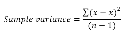
The sample variance is calculated using this formula:
Where:
- xˉ is the mean (average) of the sample values.
- n is the sample size, i.e., the number of values in the sample.
There are 3 functions to find the sample variance in Excel: VAR(), VAR.S(), and VARA().
VAR() Function in Excel
This is the oldest function in Excel to estimate variance from a sample. It is available in all versions of Excel from 2000 to 2019.
Syntax:
=VAR(number1, [number2], …)In Excel 2010, the VAR() function was replaced by VAR.S() for improved accuracy. While VAR() is still available for backward compatibility, it is recommended to use VAR.S() in current versions of Excel.
VAR.S() Function in Excel
This is the modern equivalent of the VAR() function. Use VAR.S() to find the sample variance in Excel 2010 and later versions.
Syntax:
=VAR.S(number1, [number2], …)VARA() Function in Excel
The VARA() function returns the sample variance based on a range of numbers, text, and logical values, as shown in the table earlier.
Syntax:
=VARA(value1, [value2], …)Example Variance Formula
When working with a set of numerical data, you can use any of the above functions to calculate the sample variance in Excel.
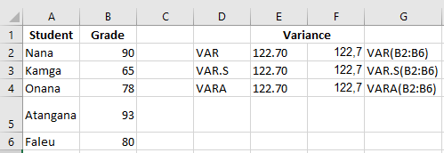
For example, let’s find the variance of a sample consisting of 5 values (B2:B6). You can use one of these formulas:
- =VAR(B2:B6)
- =VAR.S(B2:B6)
- =VARA(B2:B6)
As shown in the screenshot, all formulas return the same result (rounded to 2 decimal places).
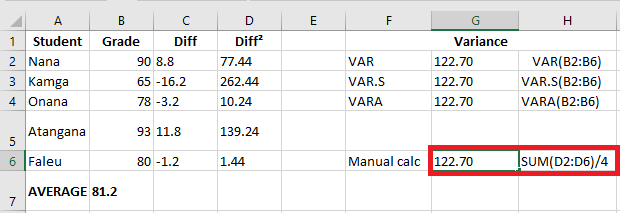
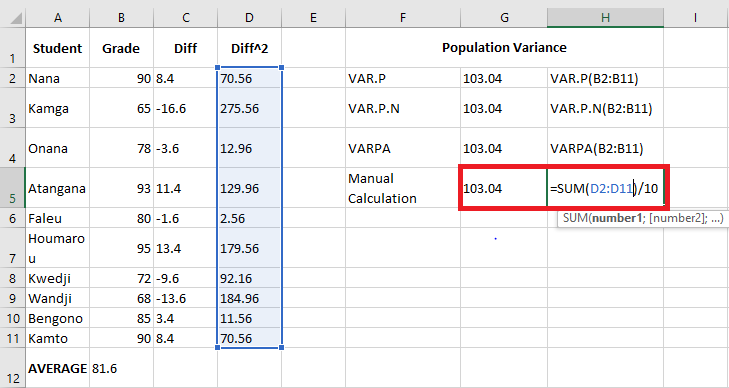
To verify the result, let’s calculate the variance manually:
- Find the mean using the AVERAGE() function:
=AVERAGE(B2:B6)
The mean goes to any empty cell, say B7. - Subtract the mean from each number in the sample:
=B2-$B$7
The differences go into column C, starting from C2. - Square each difference and place the results in column D, starting from D2:
=C2^2 - Sum the squared differences and divide by the number of elements in the sample minus 1:
=SUM(D2:D6)/(5-1)
As you can see, the result of our manual variance calculation matches exactly with the number returned by the built-in Excel functions.
If your dataset contains Boolean and/or textual values, the VARA() function will return a different result. The reason is that VAR() and VAR.S() ignore any values other than numbers in the references, while VARA() evaluates text values as zero, TRUE as 1, and FALSE as 0. Therefore, carefully choose the variance function based on whether you want to handle or ignore text and logical values.
How to Calculate Population Variance
The population refers to the entire set of observations in the area of study. The population variance describes the spread of data points in the entire population.
Population variance can be found using this formula:
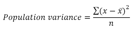
Where:
- x¯ is the population mean.
- n is the population size, i.e., the total number of values in the population.
There are 3 functions to calculate the population variance in Excel: VAR.P(), VAR.P.N(), and VARPA().
VAR.P() Function in Excel
The VARP() function returns the variance of a population based on the complete set of numbers. It is available in all versions of Excel from 2000 to 2019.
Syntax:
=VAR.P(number1, [number2], …)In Excel 2010, VARP() was replaced by VAR.P(), but it’s still kept for backward compatibility. It is recommended to use VAR.P() in current versions of Excel since there’s no guarantee that VARP() will be available in future versions.
VAR.P.N() Function in Excel
This is an enhanced version of the VAR.P() function available in Excel 2010 and later versions.
Syntax:
=VAR.P.N(number1, [number2], …)VARPA() Function in Excel
The VARPA() function calculates the variance of a population based on the complete set of numbers, text, and logical values.
Syntax:
=VARPA(value1, [value2], …)Example Population Variance Formula
In the example where we calculated the sample variance, we had 5 exam scores, assuming they were a selection from a larger group of students. If you collect data on all the students in the group, these data will represent the entire population, and you’ll calculate population variance using the functions above.
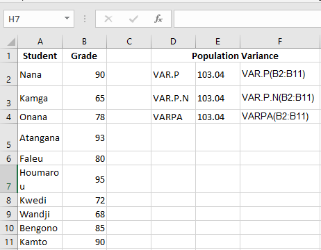
Let’s say we have the exam scores of a group of 10 students (B2:B11). The scores represent the population, so we’ll calculate the population variance using these formulas:
- =VAR.P(B2:B11)
- =VAR.P.N(B2:B11)
- =VARPA(B2:B11)
All formulas will return the identical result.
Variance Formula in Excel – Notes on Usage
To perform variance analysis correctly in Excel, please follow these simple rules:
- Provide arguments as values, arrays, or cell references.
- In Excel 2007 and later versions, you can provide up to 255 arguments for a sample or population; in Excel 2003 and earlier versions, up to 30 arguments.
- To evaluate only numbers in references, ignoring empty cells, text, and logical values, use VAR() or VAR.S() for sample variance and VAR.P() or VAR.P.N() for population variance.
- To evaluate logical and text values in references, use VARA() or VARPA().
- Provide at least two numerical values for a sample variance formula and at least one numerical value for a population variance formula in Excel, or you will get a #DIV/0! error.
- Arguments containing text that cannot be interpreted as numbers will cause #VALUE! errors.
Variance is undoubtedly a useful concept in science, but it provides very little practical information. For example, we found the ages of the tiger population in a zoo and calculated the variance, which equals 16. The question is: how can we really use this number?
You can use variance to calculate the standard deviation, which is a much better measure of the amount of variation in a dataset. The standard deviation is calculated as the square root of the variance. So, taking the square root of 16 gives a standard deviation of 4.
When combined with the mean, the standard deviation can tell you the age of most of the tigers. For example, if the mean is 8 and the standard deviation is 4, most of the tigers in the zoo are between 4 years (8 – 4) and 12 years (8 + 4).
Standard Error of the Mean (SEM) Calculation in Excel
The standard error of the mean (SEM), often abbreviated as the standard error (SE), is a measure of how much the sample mean is likely to vary from the population mean.
In other words, SEM measures the degree of variation between different samples taken from the same population, and it tells you how precisely the sample mean represents the true population mean. More broadly, the standard error indicates the degree of error you can expect in the sample mean when repeated samples are taken from the same population.
Mathematically, the standard error of the mean is typically calculated as the ratio of the standard deviation (SD) to the square root of the sample size (n):

Where σ is the standard deviation and n is the number of observations in the sample.
Excel provides an easy way to calculate the SEM using a combination of three functions, which we’ll discuss in more detail.
Importance of Calculating the Standard Error
When taking multiple samples from the same data set, calculating the standard error of the mean is important because it provides an estimate of the reliability of the sample means. A smaller standard error indicates that the sample means are more likely to be close to the true population mean, while a larger standard error suggests greater uncertainty in the estimates. Thus, the smaller the SEM, the more you can trust the accuracy of the sample mean.
The SEM is particularly useful in scientific research because it can be used to test hypotheses and determine the statistical significance of results. For example, researchers can compare sample means from two groups and calculate the SEM to determine whether the difference between the groups is likely due to chance or reflects a true difference within the population.
In summary, by providing a measure of the accuracy and precision of sample estimates, the standard error helps researchers draw more meaningful conclusions from their data. It guides decisions on sample size and statistical power, leading to more robust and reliable research outcomes.
Calculating the Standard Error of the Mean in Excel
Since the standard error is equal to the standard deviation divided by the square root of the sample size, Excel provides a simple way to calculate the SEM using three different functions.
Here’s how you can calculate the standard error of the mean in Excel:
- Enter your data in an Excel worksheet, organizing them in rows or columns.
- Calculate the sample standard deviation using the function STDEV.S.
- Find the sample size (the total number of values) using the COUNT function.
- Find the square root of the sample size using the SQRT function.
- Divide the standard deviation by the square root of the sample size.
The generic formula to calculate SEM in Excel is:
=STDEV.S(range)/SQRT(COUNT(range))
Where range refers to the range of cells containing your data.
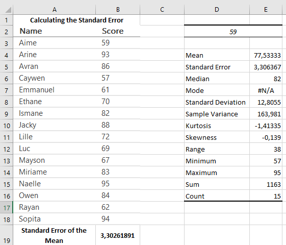
For example, if your data range is from B2:B18, the SEM formula in Excel would look like this:
=STDEV.S(B2:B18)/SQRT(COUNT(B2:B18))
Once the formula is calculated, the result will appear as the standard error of the mean.

Finding the Standard Error Using the Analysis ToolPak
Another way to calculate the standard error of the mean in Excel is by using the Analysis ToolPak. To use this feature, you first need to ensure that the ToolPak add-in is installed in your Excel. Below are the steps to activate the Analysis ToolPak add-in in Excel.
Activating the Analysis ToolPak
With the Analysis ToolPak add-in enabled, you can calculate the standard error of the mean by following these steps:
-
Enter your sample data into a single column.
-
Go to the Data tab, and in the Analysis group, click on Data Analysis.

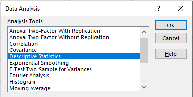
-
In the Data Analysis dialog box, select Descriptive Statistics from the list of analysis tools and click OK.
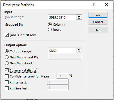
In the Descriptive Statistics dialog box, proceed as follows:
-
In the Input Range field, select the range of cells containing your sample data.
-
If you included column headers in your selection, make sure to check the box labeled « Labels in first row » to ensure the data is analyzed correctly.
-
In the Output Range section, choose where you want the results to appear. To avoid overwriting existing data, it’s safer to select New Worksheet Ply. If you prefer to display the results on the same sheet, choose the top-left cell of an empty area and ensure there’s at least one empty column to the right.
-
Check the box next to Summary statistics, and click OK.
Excel will now generate a new table containing various descriptive statistics for your sample data, including the standard error of the mean. You can verify that the standard error value exactly matches the SEM (Standard Error of the Mean) calculated using the formula, as shown in the screenshot below.
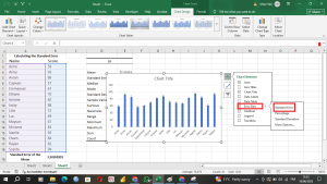
Adding Standard Error Bars in Excel
To visually display the variability of data points and highlight the precision of the sample mean, you can add standard error bars to an Excel chart. The standard error bars show the range of values within which the sample mean is likely to fall, given a specific confidence level.
To add standard error bars to an Excel chart, follow these steps:
- Create a chart from your data. Select the data range, go to the Insert tab, and choose the desired chart type from the Charts group.
- Select the chart, then click the Chart Elements button at the top right of the chart.
- In the dropdown menu, click the arrow next to Error Bars and select Standard Error.
The standard error bars will be added to your chart, helping you compare the means across different groups and assess the significance of any observed differences.
Standard Error of the Mean vs. Standard Deviation
The standard deviation and the standard error of the mean are two related statistical concepts that are often used to measure the variability of data. Although they may seem similar, they have different meanings and uses.
- Standard Deviation (SD) measures the amount of variation or dispersion in a data set from its mean. A high standard deviation indicates that the data points are spread out far from the mean, while a low standard deviation suggests that the data points are closer to the mean.
- Standard Error of the Mean (SEM) measures the variability of the sample mean compared to the population mean. The standard error indicates how accurately the sample mean represents the true population mean, and it reflects the degree of error expected when taking multiple samples from the same population. A low SEM suggests that the sample mean is a good estimate of the population mean, while a high SEM suggests that the sample mean may not be a reliable estimate of the population mean.
The standard error of the mean is always smaller than the standard deviation because it is calculated by dividing the standard deviation by the square root of the sample size, which reduces its value.

In Summary:
- The standard deviation measures variability within a dataset, while the standard error of the mean measures how much the sample mean is likely to vary from the true population mean.
- Excel provides simple ways to calculate SEM, either through functions like STDEV.S and SQRT or using the Analysis ToolPak for more detailed descriptive statistics.
- SEM is particularly useful for estimating the precision of sample means and is often used in scientific research to assess the reliability of data.
Mode Calculation in Excel
The mean provides a measure of central tendency by considering all the actual values in a group. The median measures central tendency differently, providing the midpoint of a sorted group of values. The mode takes another approach: it tells you which of several values occurs most frequently. While the mean and median require certain calculations, a mode value can be found simply by counting how many times each value occurs.
For example, the mode of the dataset {1, 2, 2, 3, 4, 6} is 2. In Microsoft Excel, you can calculate the mode using the function of the same name: MODE. For our example dataset, the formula would be:
=MODE(B2:B10)
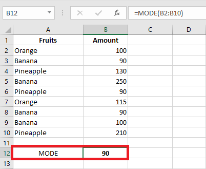
In situations where there are two or more modes in your dataset, the Excel MODE function will return the lowest mode.
Determining the Mode of Nominal Data Using Pivot Tables
However, the MODE() function does not work with nominal data. If you present it with a range that contains only text data such as names, MODE() will return the #N/A error. If one or more text values are included in a list of numerical values, MODE() simply ignores the text values.
In such cases, pivot tables can be a helpful alternative to find the mode. Here is a quick overview of the process:
- Prepare Your Data: Arrange your raw data in a list format in Excel. The field name in the first column (like A1) and the values in the cells below (like A2:A21). It’s better if all cells adjacent to the list are empty.
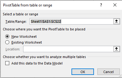
- Insert a Pivot Table:
- Click on the Insert tab on the ribbon, then select Pivot Table in the Charts group.
- Excel will automatically populate the range in the Table/Range field if you selected a cell in your list before clicking Pivot Table.
- Configure Your Pivot Table:
- Place the field(s) you’re interested in into the Rows and Values areas of the PivotTable Field List.
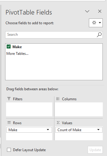
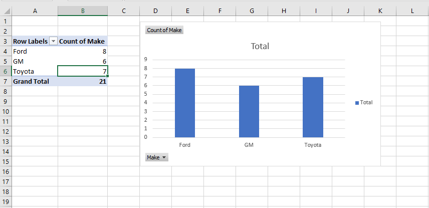
The PivotTable will now show the frequency distribution, where the mode is the value that occurs most often.
Comments on the Mode Analysis
- The mode is a very useful statistic when applied to categories such as political parties, popular brands, weekdays, and regions. Excel should have an integrated function for the mode of text values. While it doesn’t, the next section will show you how to write your own formula for the mode that works with both numerical and text values.
- When you only have a few distinct categories, consider creating a pivot table to show the count of each category. A pivot table that shows the count of instances of each category is an attractive way to present your data to an audience.
- Standard Excel charts don’t show the number of instances per category without prior work. You should count each category before creating the chart, which is the purpose of the PivotTable supporting the PivotChart. The PivotTable is simply a faster way to perform the analysis than manually creating a table for counting category membership and then building a standard Excel chart based on it.
- The mode is the only sensible measure of central tendency when working with nominal data such as category names. The median requires sorting things in some way: from shortest to longest, cheapest to most expensive, or slowest to fastest. In terms of scale types, you need at least an ordinal scale to get a median, and many categories are nominal, not ordinal. Variables represented by values like Ford, GM, and Toyota don’t have a meaningful mean or median.
Getting the Mode of Categories with a Formula
The MODE() function in Excel doesn’t work when you provide text values as arguments. Here’s a method to get the mode using a formula. This formula will tell you which text value appears most frequently in your dataset. You’ll also learn how to create a formula to count the number of instances of the existing mode.
If you don’t want to use a PivotChart to find the mode of a group of text values, you can find it using the following formula:
=INDEX(A2:A21, MODE(MATCH(A2:A21, A2:A21, 0)))
Assuming the text values are in A2:A21 (the range could occupy a single column like A2:A21 or a single row like A2:Z2, but it won’t work properly with a multi-column range like A2:Z21).
If you’re new to Excel, this formula may look confusing. I’ve structured it based on my long experience with Excel, and I still need to pause and think about it before I can explain why it returns the mode. So, don’t worry if it seems puzzling right now. Over time, it will become clearer, and for now, you can use it to get the modal value for any set of text values in a worksheet.
Formula breakdown:
- The MATCH() function returns the position in the array where each value first appears. The third argument of MATCH() is set to 0, meaning an exact match is required, and the array doesn’t need to be sorted. So, for every instance of Ford in the values array A2:A21, MATCH() returns 1; for every instance of Toyota, it returns 2; and for GM, it returns 4.
- The results of the MATCH() function are used as an argument for the MODE() function. In this example, MODE() evaluates 20 values: some equal 1, some equal 2, and others equal 4. MODE() returns the most frequent of these numbers.
- The result of MODE() is then used as the second argument for the INDEX() function. The first argument is the array to check. The second argument tells INDEX() how far to look in the array. Here, it looks at the first value, which is Ford. If GM had been the most frequent text value, MODE() would have returned 4, and INDEX() would have used that value to find GM in the array.
Using an Array Formula to Count the Values
Once you have the modal value (Ford in this example), you still want to know how many instances of this mode exist. This section describes how to create the array formula to count the instances.
For this, use the following formula:
=SUM(IF(A2:A21 = C1, 1, 0))
This is an array formula and must be entered using the special key combination Ctrl + Shift + Enter. You’ll know it’s an array formula if you see curly braces around it in the formula bar.
Formula breakdown:
- The A2:A21 = C1 part checks whether each value in the range A2:A21 equals the value in cell C1 (Ford in this example).
- This results in a TRUE or FALSE array.
- The IF() function then converts these values: TRUE becomes 1 and FALSE becomes 0.
- The SUM() function adds up all the 1s (the instances of the mode).
For example, if Ford is the mode, the formula will count how many times Ford appears in the range A2:A21.
Recap of the Array Formula
To summarize how the array formula counts values for the modal category Ford, consider the following:
- The goal is to count how many times Ford appears in the range A2:A21.
- The A2:A21 = C1 part creates a TRUE/FALSE array depending on whether each cell matches Ford.
- The IF() function turns TRUE into 1 and FALSE into 0.
- The SUM() function adds up the 1s and 0s, giving the count of instances of Ford.
This array formula efficiently counts occurrences of the modal value in a given range.
Median Calculation in Excel
The median is one of the three main measures of central tendency, widely used in statistics to identify the center point of a dataset or population. It provides a useful summary when analyzing values such as typical salaries, household incomes, property prices, land taxes, and other economic indicators.
What is the Median?
Simply put, the median represents the middle value in a sorted set of numbers. It divides the dataset into two equal halves — one containing values lower than the median and the other containing values higher than the median.
When the dataset contains an odd number of elements, the median is the middle value. However, when the dataset has an even number of elements, the median is calculated as the average of the two middle values.
For example:
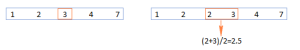
- In the dataset {1, 2, 3, 4, 7}, which contains five elements, the median is 3, because it is the third and central value in the ordered list.
- In the dataset {1, 2, 2, 3, 4, 7}, which has six elements, the two middle values are 2 and 3, so the median is their average: (2 + 3) / 2 = 2.5.
I
Unlike the arithmetic mean (average), the median is much less affected by outliers—values that are significantly higher or lower than the rest of the data. This makes the median the preferred measure of central tendency when dealing with skewed distributions or datasets with extreme values.
A classic example is median salary. It provides a more accurate picture of what most people earn compared to the average salary, which can be misleading if a small number of individuals earn exceptionally high or low salaries. In such cases, the average can be heavily distorted, while the median remains a more reliable indicator of the typical income.
The MEDIAN Function in Excel
Microsoft Excel includes a built-in function called MEDIAN to calculate the median of a set of numeric values efficiently. The syntax of the MEDIAN function is as follows:
=MEDIAN(number1, [number2], …)- number1, number2, … are the numeric values or references for which you want to find the median.
- These can be hardcoded numbers, dates, named ranges, arrays, or cell references containing numbers.
- The first argument (number1) is required, while the remaining arguments are optional.
In Excel 2007 and later versions (including Excel 2010, 2013, 2016, and beyond), the MEDIAN function supports up to 255 arguments. In older versions like Excel 2003 and earlier, it can handle up to 30 arguments.
Four Key Facts About the MEDIAN Function
Here are four important behaviors to understand when using the MEDIAN function:
- Odd vs Even Count: If the number of values is odd, the function returns the middle value. If the number is even, it returns the average of the two middle values.
- Zero Values: Cells containing the number 0 are included in the calculation.
- Empty and Non-Numeric Cells: Blank cells, cells with text, or cells containing logical values like TRUE or FALSE (when referenced via a range) are ignored.
- Logical Values in Arguments: If logical values (TRUE or FALSE) are entered directly as arguments, they are included. For example:
=MEDIAN(FALSE, TRUE, 2, 3, 4)
Excel interprets FALSE as 0 and TRUE as 1, so the dataset becomes {0, 1, 2, 3, 4}. The median is 2.
How to Calculate the Median in Excel: Formula Examples
The MEDIAN function is one of the simplest and most user-friendly statistical functions in Excel. Still, there are some useful tricks that beginners may not immediately discover—such as calculating the median based on a condition (which will be covered in more advanced examples).
Let’s start with the basic use of the function. Suppose you have a sales report and want to find the median of the sales values in cells C2 to C8. You can use the following straightforward formula:
=MEDIAN(C2:C10)
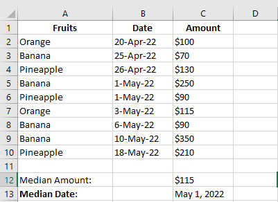
As demonstrated in the screenshot above, the MEDIAN function works seamlessly with both numbers and dates, since Excel internally treats dates as serial numbers. This means that you can calculate the median of a set of dates in the same way you would for numerical values.
Conditional Median Formula Based on a Single Criterion
Unfortunately, Microsoft Excel does not offer a built-in function to calculate a conditional median (like it does for the average using
AVERAGEIF()orAVERAGEIFS()). However, you can easily create your own custom array formula to perform this calculation.The general structure of the conditional median formula is:
=MEDIAN(IF(criteria_range = criteria_value, median_range))
Example:
Suppose you have a table with the following columns:
- Column A: Item Name
- Column C: Amount
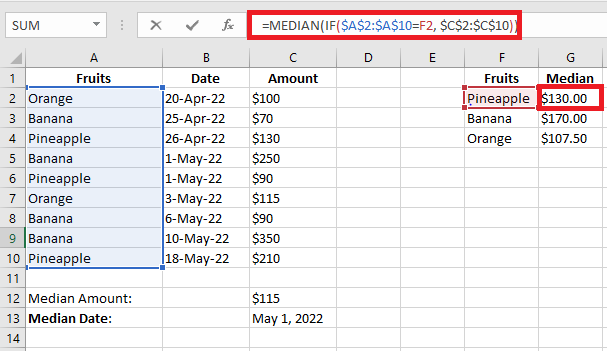
To calculate the median amount for a specific item (e.g., « Apples »), first enter the item name (e.g., « Apples ») in a cell, say E2, and then use the following formula:
=MEDIAN(IF($A$2:$A$10 = $E$2, $C$2:$C$10))
This formula tells Excel to:
- Look at all the values in Column A (items) from cells A2 to A10.
- Compare each one with the value in cell E2 (e.g., « Apples »).
- Only if there is a match, include the corresponding value from Column C (amount) in the median calculation.
Important Notes:
- The dollar signs (
$) are used to make the cell references absolute, so they don’t change when you copy the formula to other cells. - Because the
IF()function returns an array, this formula must be entered as an array formula in Excel versions prior to Office 365 or Excel 2021.
To do this:- Press Ctrl + Shift + Enter instead of just Enter.
- If done correctly, Excel will display the formula enclosed in curly braces
{}like this:
In Excel 365 and Excel 2021 (with dynamic arrays), pressing just Enter is sufficient.
Conditional Median Formula Based on Multiple Criteria
To take the previous example a step further, suppose you add an additional column to your dataset, such as Order Status. You now want to calculate the median amount for each item, but only for orders that match a specific status (e.g., « Completed »).
In other words, we are calculating the median based on two conditions:
-
The Item Name
-
The Order Status
Since Excel does not offer a built-in
MEDIANIFS()function, you can use nestedIFstatements inside theMEDIANfunction to simulate this behavior.General Formula Syntax:
=MEDIAN(IF(criteria_range1 = criteria1, IF(criteria_range2 = criteria2, median_range)))
This structure allows you to filter the data by multiple conditions before calculating the median.
Example:
Assume your table contains the following columns:
-
Column A: Item Names (e.g., « Apple », « Banana »)
-
Column C: Order Amounts
-
Column D: Order Status (e.g., « Pending », « Completed »)
Now, to calculate the median for a given item and status:
-
Enter the item name in cell F2 (e.g., « Apple »)
-
Enter the order status in cell G2 (e.g., « Completed »)
Then use the following formula:
=MEDIAN(IF($A$2:$A$10 = $F2, IF($D$2:$D$10 = $G2, $C$2:$C$10)))
Important Notes:
-
This is an array formula, so in older versions of Excel (prior to Excel 365 or Excel 2021), you must confirm it by pressing Ctrl + Shift + Enter instead of just Enter.
- If done correctly, Excel will display the formula wrapped in curly braces:
{=MEDIAN(IF($A$2:$A$10 = $F2, IF($D$2:$D$10 = $G2, $C$2:$C$10)))}-
In Excel 365 and later, you can simply press Enter thanks to dynamic array support.
This method enables you to compute the conditional median with multiple criteria, which is especially useful in complex datasets—for example, calculating the median value of all « Banana » orders that are currently « Completed », excluding all others
Median vs Mean: Which Is the Best Measure?
Generally, there is no “best” measure of central tendency. The measure to use mainly depends on the type of data you’re working with and your understanding of the « typical value » you’re trying to estimate.
- For a symmetric distribution (where values appear at regular frequencies), the mean, median, and mode are the same.
- For an asymmetric distribution (where there are a few extremely high or low values), these three measures can be different.
Since the mean is heavily influenced by outliers (values that are significantly different from the rest of the data), the median is often the preferred measure for skewed distributions.
For example, the median is generally considered a better measure than the mean when calculating a « typical salary. » Why? The best way to understand this would be through an example. Let’s consider the following salaries for common jobs:
- Electrician – $20/hour
- Nurse – $26/hour
- Police Officer – $47/hour
- Sales Manager – $54/hour
- Manufacturing Engineer – $63/hour
Now, calculate the mean (average):
(20 + 26 + 47 + 54 + 63) / 5 = 42. So, the average salary is $42/hour. The median salary is $47/hour (the police officer earns this). So, half earn less and half earn more.Now, let’s say we add a celebrity earning around $30 million a year, or about $14,500/hour. The new average salary becomes $2,451.67/hour, a salary that nobody earns! However, the median remains largely unchanged at $50.50/hour.
As you can see, the median provides a better idea of what people typically earn because it’s not so strongly affected by outliers like extremely high salaries.
Conclusion
That’s how you calculate the mean, median, and mode in Excel. I hope you find this useful for your data analysis tasks! Thank you for reading, and I look forward to seeing you on our blog next week!
Weighted Average Calculation in Excel
Although Microsoft Excel does not provide a specific weighted average function, it has several other functions that can be used to perform this calculation, as shown in the examples below.
What is a Weighted Average?
A weighted average is a type of arithmetic average where some elements in the data set carry more importance than others. In other words, each value being averaged is assigned a certain weight.
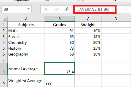
Student grades are often calculated using a weighted average. For example, a regular average is easily calculated using Excel’s AVERAGE() function. However, when we need the average to account for the weight of each activity listed in column C, a weighted average formula is necessary.
In mathematics and statistics, the weighted average is calculated by multiplying each value in the set by its respective weight, then adding these products together and dividing the sum of the products by the sum of all the weights.
For instance, to calculate the weighted average (overall grade), you multiply each score by its corresponding percentage (converted to decimal form), sum the 5 products, and then divide by the sum of the 5 weights:
((91*0.1)+(65*0.15)+(80*0.2)+(73*0.25)+(68*0.3)) / (0.1+0.15+0.2+0.25+0.3) = 73.5
As you can see, the regular average (75.4) and the weighted average (73.5) are different values.
Calculating the Weighted Average
In Microsoft Excel, you can calculate the weighted average using the same approach but with much less effort, as Excel’s functions will do most of the work for you.
Example 1: Calculating the Weighted Average Using the SUM() Function
If you are familiar with the basic SUM() function in Excel, the formula below will require little explanation:
=SUM(B2*C2, B3*C3, B4*C4, B5*C5, B6*C6) / SUM(C2:C6)
Essentially, it performs the same calculation as described above, but using cell references instead of numbers.
As shown in the screenshot, the formula returns exactly the same result as the previous manual calculation. Notice the difference between the regular average (calculated using AVERAGE() in C8) and the weighted average (calculated in C9).
Although the SUM() formula is simple and easy to understand, it’s not the best choice if you have a large number of elements to average. In this case, you should use the SUMPRODUCT() function as shown in the next example.
Example 2: Finding a Weighted Average with the SUMPRODUCT() Function
Excel’s SUMPRODUCT() function is perfect for this task as it is designed to sum products, which is exactly what we need. Instead of multiplying each value by its weight individually, you provide two arrays in the SUMPRODUCT() formula (in this context, an array is a continuous range of cells), then divide the result by the sum of the weights:
=SUMPRODUCT(values_range, weights_range) / SUM(weights_range)
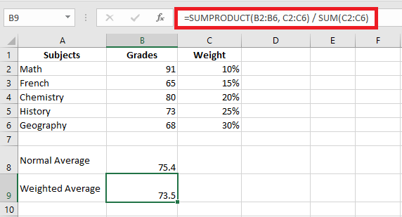
Assuming the values to be averaged are in cells B2:B6 and the weights are in cells C2:C6, our SUMPRODUCT() formula for the weighted average looks like this:
=SUMPRODUCT(B2:B6, C2:C6) / SUM(C2:C6)
To view the actual values behind an array, select it in the formula bar and press the F9 key. The result will look something like this:
=SUMPRODUCT(91*0.1 + 65*0.15 + 80*0.2 + 73*0.25 + 68*0.3)
What the SUMPRODUCT() function does is multiply the 1st value in array1 by the 1st value in array2 (910.1 in this example), then multiply the 2nd value in array1 by the 2nd value in array2 (650.15), and so on. After all multiplications are done, the function adds the products and returns that sum.
To ensure the SUMPRODUCT() function gives the correct result, you can compare it to the SUM() formula from the previous example, and you’ll find the numbers are identical.
Excel’s SUM() or SUMPRODUCT() for Weighted Averages
- The weights don’t necessarily need to add up to 100%, and they don’t have to be expressed as percentages.
- For example, you can create a priority scale and assign a certain number of points to each item, just like in the example above.
With these formulas, you can easily calculate a weighted average in Excel without manually multiplying and adding each value. Excel’s functions will handle most of the heavy lifting for you.