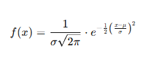
A T-test is a fundamental statistical method used to determine whether there is a significant difference between the means of two groups, which may or may not be related. This test helps assess whether the observed differences in sample means reflect actual differences in the populations they represent, or whether they occurred by random chance.
The T-test works by analyzing randomly selected samples from the two groups or categories being compared. It is particularly useful when the population data does not perfectly follow a normal distribution, which is often the case in real-world data.
The type of T-test to be applied depends on the nature of the samples being studied—whether they are independent or paired, and whether the variances are assumed to be equal or unequal. The result of the test helps estimate the probability (p-value) that the observed difference in means occurred by chance.
T-tests are commonly used in a wide variety of contexts, such as:
-
Comparing the average age between two population groups,
-
Evaluating the growth duration of two different crop species,
-
Analyzing student performance across different teaching methods or classes
Understanding the T-Test
A T-test is a statistical method used to evaluate data collected from two similar or distinct groups to determine the probability that the observed difference in results occurred by chance. It helps answer whether the variation in outcomes between groups is statistically significant or simply due to random variation.
The accuracy of a T-test relies on several factors, such as the underlying data distribution, sample size, and variability within the samples. Based on these factors, the test produces a T-value, which serves as a statistical indicator of the likelihood that the observed difference is due to chance.
Example:
Suppose a researcher wants to assess whether the average petal length of a flower differs between two species. The researcher can randomly collect petal length data from both species and conduct a T-test to statistically compare the two means. The conclusion is then drawn based on the resulting T-value and corresponding p-value.
The interpretation of the T-test result usually follows two hypotheses:
- Null Hypothesis (H₀): Assumes that there is no difference between the means of the two groups (i.e., the means are equal).
- Alternative Hypothesis (H₁): Assumes that the means are significantly different, implying that the difference is not due to random chance, and the null hypothesis is rejected.
Note: A T-test is only appropriate when comparing two groups. If more than two groups need to be compared simultaneously, an ANOVA (Analysis of Variance) test is more appropriate.
T-Test Assumptions
For a T-test to yield valid results, several assumptions must be met:
- Scale of Measurement: The data should be measured on an interval or ratio scale. Continuous or ordinal patterns must be followed when setting up hypotheses.
- Random Sampling: Data should be obtained through a process of random sampling. Since individual identity is not preserved, the reliability depends on how representative the sample is.
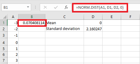
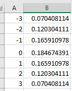
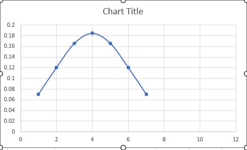
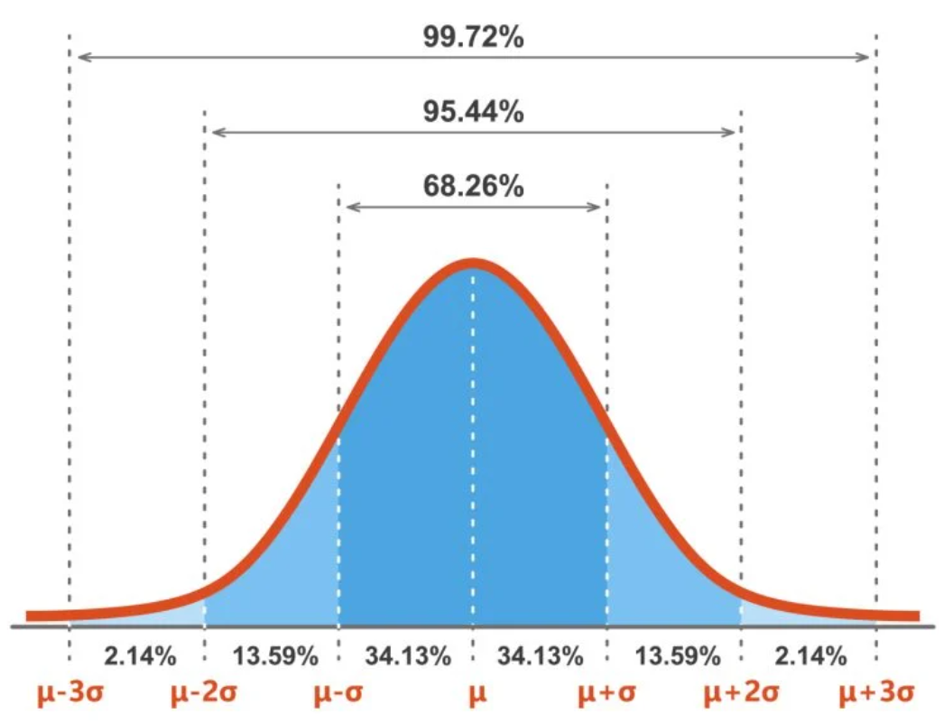
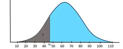
- Normality: The distribution of the sample data should approximate a normal distribution. When plotted, the data should ideally form a bell-shaped curve.
- Sample Size: A larger sample size helps achieve a more clearly defined normal distribution curve, enhancing test reliability.
- Homogeneity of Variance: The standard deviations of the groups being compared should be approximately equal. If this assumption is violated, a different version of the T-test (Welch’s T-test) should be used.
Types of T-Tests
There are several commonly used types of T-tests, depending on the nature of the data and comparison:
One-Sample T-Test
This test compares the mean of a single group to a known or hypothesized population mean. It helps determine whether the sample differs significantly from a set benchmark.
Example:
A teacher wants to determine if the average weight of 5th-grade students is greater than 45 kg.
- She randomly selects a group of students, records their individual weights, and calculates the sample mean.
- Then, she uses a one-sample T-test to check if the sample mean is statistically different from 45 kg.
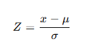
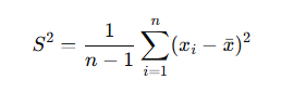
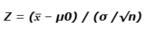
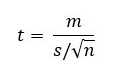
Formula (for a one-sample T-test):
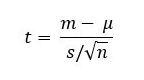
Where:
- xˉ = sample mean
- μ = population mean
- s = sample standard deviation
- n = sample size
Independent Two-Sample T-Test
The independent two-sample T-test, also known as the independent T-test, is used to compare the means of two independent groups or populations. This test is appropriate when the samples come from different groups that are unrelated to each other.
Example:
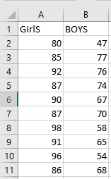
A teacher wants to compare the average height of male and female students in Grade 5. Since these are two separate groups, an independent two-sample T-test is used.
Formula:
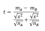
Where:
- mA−mB = difference between sample means
- nA, nB = sample sizes of groups A and B
- s2 = pooled variance (assuming equal variances)
Paired Sample T-Test
A paired sample T-test is used when two measurements are taken from the same group at different times or under two different conditions. It accounts for the fact that the data points are not independent but related or « paired. »
Example:
A nutritionist measures the weight of a group of individuals before and after a diet plan. Since the same individuals are measured twice, the data are paired.
Formula:
Where:
- m = mean of the differences between paired observations
- s = standard deviation of the differences
- n = number of pairs
This test determines whether the average change is statistically significant.
Equal Variance T-Test (Pooled T-Test)
This version of the T-test is applied when the sample sizes are equal or nearly equal, and the variances of the two groups are assumed to be approximately the same. It is sometimes referred to as the pooled T-test.
Formula:
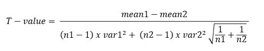
Where:
-
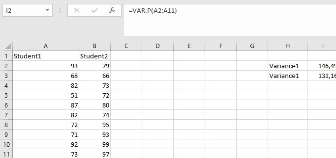
Mean1 and Mean2 = the mean value of each sample set
-
Var1 and Var2 = the variance of each sample set
-
n1 and n2 = the number of records (sample size) in each set
Unequal Variance T-Test (Welch’s T-Test)
The Welch’s T-test is used when the variances and sample sizes differ significantly between the two groups. It is a robust alternative to the standard T-test and does not assume equal variances.
Formula:
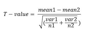
Where:
-
-
Mean1 and Mean2 = the mean value of each sample set
-
Var1 and Var2 = the variance of each sample set
-
n1 and n2 = the number of records (sample size) in each set.
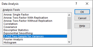
Performing a T-Test in Excel
A T-test in Excel can be conducted using either the Data Analysis Toolpak or the T.TEST function. Note that the older TTEST function has been replaced by T.TEST starting with Excel 2010 and onwards.
The T.TEST function, also referred to as TEST.STUDENT in certain language settings, is categorized under Excel’s statistical functions and is used to determine the probability associated with a Student’s T-Test.
Syntax of the T.TEST Function
Where:
-
array1 – This is the first range of data (sample set) on which the T-test will be performed.
-
array2 – This is the second range of data to be compared against the first.
-
tails – Specifies the number of distribution tails. It can be:
-
1 – for a one-tailed test: Used when testing if the mean of one group is greater or less than the other in a specific direction.
-
2 – for a two-tailed test: Used when testing if the means of the two populations are significantly different, regardless of direction.
-
type – Indicates the type of T-test to be performed. It can be:
-
1 – Paired T-test (used when comparing two related samples, such as measurements before and after treatment).
-
2 – Two-sample equal variance T-test (used when the two samples are independent and assumed to have equal population variances — i.e., homoscedastic).
-
3 – Two-sample unequal variance T-test (also known as Welch’s test, used when the two independent samples are assumed to have unequal variances — i.e., heteroscedastic).
All arguments are required when using the T.TEST function in Excel.
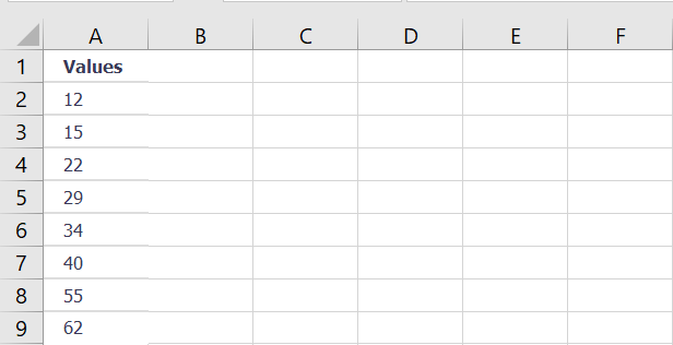
Example 1 – Paired Sample T-Test Using a One-Tailed Distribution
Suppose we want to test whether there is a statistically significant difference in spending (in INR) by an organization between two countries — India and the United States — using paired data (e.g., corresponding monthly expenditures over the same period).
Steps to perform the T-test:
-
In Excel, assume:
- To perform a paired one-tailed T-test, enter the following formula in cell B25:
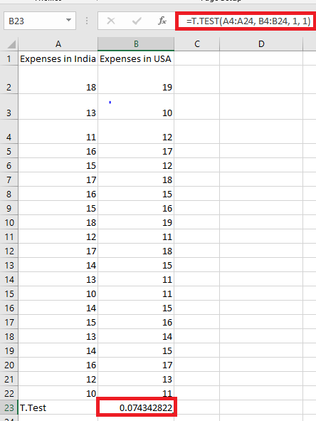
Press the “Enter” key.
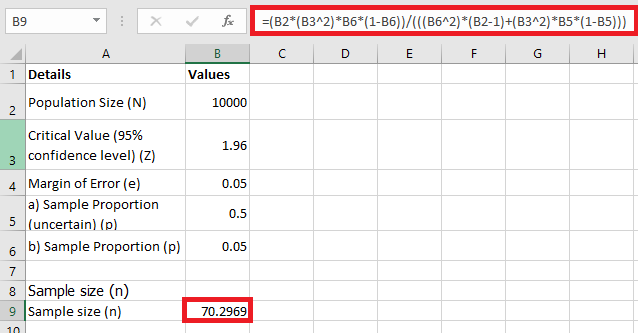
The output in cell B25 is 0.074342822, as shown in the image below.
One-tailed/Two-tailed Explanation:
The range A4:A24 (entered in step 1 of the formula) represents the first dataset on which the Excel t-Test is to be performed. Similarly, B4:B24 represents the second dataset.
Additionally, we entered the arguments « tails » and « type » as 1. This indicates that a one-tailed, paired t-Test is being conducted.
Interpretation:
To determine whether to accept or reject the null hypothesis, perform the following steps:
-
Compare t-Statistic with Critical t-Value:
Refer to the one-tailed t-distribution table to find the critical t-value at a given significance level (alpha), with the appropriate degrees of freedom (df).
Then compare this table value to the calculated t-statistic (0.177639611).
-
Compare p-Value with Significance Level:
Use the p-value obtained from the t-Test and compare it with the chosen significance level.
Since alpha is not specified in the question, assume it to be 0.05 (5%).
Decision-making regarding the null hypothesis should be based on both the t-value and the p-value. Rejecting the null hypothesis implies accepting the alternative hypothesis.
Note: When comparing t-values, you can ignore the negative sign (if present).
NOTE:
The null hypothesis in a paired sample t-Test in Excel assumes that the mean difference between paired observations is zero.
In other words, the average values of both paired datasets are equal.
The alternative hypothesis assumes that the mean difference is not zero.
For example, for row 4, the paired difference would be calculated as (18 – 19) or (cell A4 – cell B4).
Rejecting the null hypothesis means that a significant average difference exists between the paired observations — i.e., the average difference is not zero.
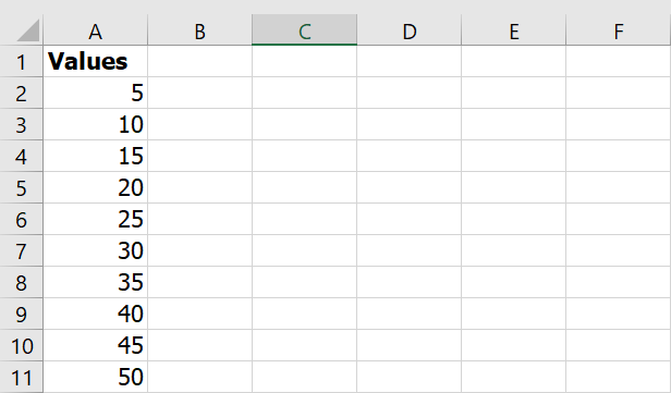
Example 2 – Two-Sample Equal Variance t-Test Using One-Tailed Distribution
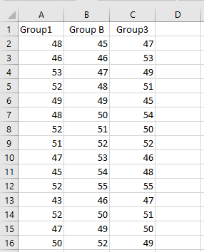
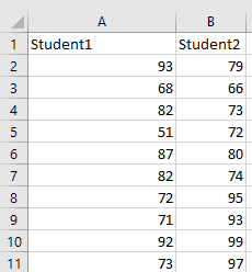
An organization launched a new beverage flavor. To test its effectiveness, two samples (each with 21 people) were created.
Assume both groups (New and Old) are independent samples and have equal population variances.
Now, perform a two-sample equal variance t-Test in Excel using a one-tailed distribution.
Steps to Perform the t-Test:
Step 1: In cell B52, enter the following formula:
=T.TEST(B2:B22, C2:C22, 2, 1)
This is shown in the image below.
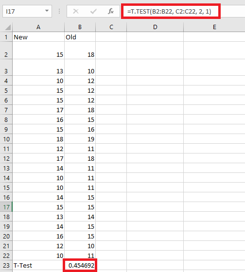
Step 2: Press the “Enter” key.
The output in cell B52 is 0.454691996.
Explanation:
-
The first data range in the formula (entered in Step 1) is A31:A51
-
The second data range is B31:B51
-
The argument 1 indicates a one-tailed test
-
The argument 2 specifies a two-sample equal variance t-Test (also known as a homoscedastic t-Test)
Interpretation:
To determine whether to accept or reject the null hypothesis, proceed as follows:
-
Compare the calculated t-statistic with the critical t-value from the t-distribution table
-
Simultaneously, compare the p-value with the standard significance level (alpha = 0.05)
t-Test Hypotheses (Equal Variance, Two-Sample):
-
Null Hypothesis (H₀):
There is no difference between the means of the two samples (i.e., the means are equal).
-
Alternative Hypothesis (H₁):
There is a difference between the sample means (i.e., the means are not equal).
NOTE:
Rejecting the null hypothesis suggests that there is a significant difference between the two sample means — and this difference is not due to random chance.
If you’re unsure whether to use the one-tailed or two-tailed t-critical values, it’s safer to compare the t-statistic against the two-tailed t-critical value for a more conservative interpretation.
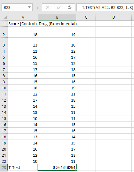
Example #3 – Two-Sample Unequal Variance t-Test Using a One-Tailed Distribution
A researcher wants to study the impact of a new drug on a person’s driving performance. A total of 21 individuals were administered the drug before taking a driving test.
The population variances of the two samples are unequal.
Perform a two-sample t-Test assuming unequal variances using a one-tailed distribution.
Steps to Perform the Test:
Step 1: Enter the following formula in cell B23:
This setup is shown in the image below.
Step 2: Press the « Enter » key on your keyboard.
As a result, the output displayed in the cell will be 0.364848284, as shown in the image below. This value corresponds to the result of the formula or operation entered in the previous step.
Explanation:
The range A2:A22 represents the first data array, as referenced in the formula entered in Step 1. The range B2:B22 represents the second data array, which will be compared to the first using Excel’s T.TEST function.
Since a one-tailed test is required, we enter 1 for the "tails" argument. The value 3 for the "type" argument specifies that Excel should perform a two-sample t-test assuming unequal variances (also known as Welch’s t-test).
Interpretation:
To interpret the result, compare the calculated t-value (returned by Excel) with the critical t-value from the t-distribution table at the chosen level of significance.
-
If the calculated t-value is greater than the critical t-value, the null hypothesis is rejected.
-
Similarly, if the p-value returned by Excel is less than the significance level (e.g., 0.05), the null hypothesis is rejected in favor of the alternative hypothesis.
NOTE:
In a two-sample t-test assuming unequal variances, the null hypothesis states that the means of the two samples are equal.
The alternative hypothesis asserts that the means are different (i.e., not equal).
Common Errors Returned by the Excel T.TEST Function:
The T.TEST function in Excel can return several types of errors depending on the input values. These include:
-
#N/A Error:
This appears when the two data arrays are of different lengths and a paired t-test is specified (type = 1).
-
#NAME? Error:
This occurs when either the "tails" or "type" argument is provided as text rather than a numeric value.
-
#NUM! Error:
This error is returned in the following cases:
-
If the "tails" argument is not 1 (one-tailed) or 2 (two-tailed).
-
If the "type" argument is not 1, 2, or 3.
For example, in the illustration provided, the error #NUM! is shown because the "tails" argument was incorrectly entered as 5, and the two data arrays were of different sizes.
Even if both arrays had the same length, using invalid values for the "tails" (e.g., 5) or "type" arguments would still result in a #NUM! error.
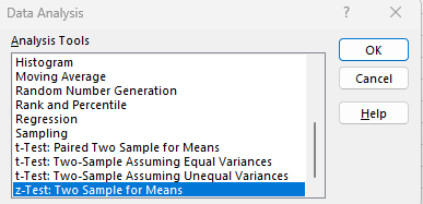
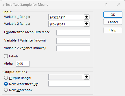
Key Differences Between the Z-Test and the T-Test
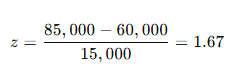
The Z-test is a statistical hypothesis test typically used to determine whether there is a significant difference between the means of two groups when the population standard deviation (or variance) is known and the sample size is large. In contrast, the T-test is employed when the population variance is unknown and is estimated using the sample data, particularly when the sample size is small.
Both Z-tests and T-tests are foundational tools in inferential statistics and are widely used across disciplines such as science, business, medicine, and social sciences. While both are univariate hypothesis tests, they differ in their underlying assumptions and applications.
Main Differences
- Knowledge of Population Variance
- The Z-test requires that the population variance or standard deviation is known or assumed to be known.
- The T-test, however, is applied when the population variance or standard deviation is unknown, and thus must be estimated from the sample.
- Distribution Assumptions
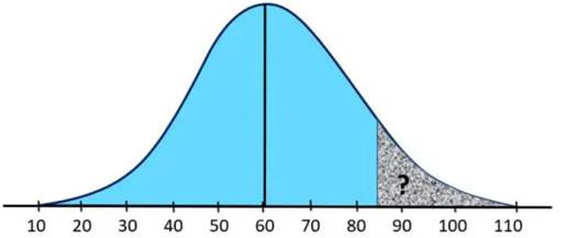
- The Z-test assumes that the sampling distribution of the sample mean follows a normal distribution.
- The T-test is based on the Student’s t-distribution, which is similar in shape to the normal distribution but has heavier tails, especially when sample sizes are small. This accounts for additional uncertainty due to estimating the population standard deviation.
- Sample Size Requirement
- The Z-test is appropriate for large samples (typically n > 30).
- The T-test is more suitable for small samples (usually n < 30), where the sampling variability is higher.
- Application Context
- The Z-test is ideal when comparing two sample means and population parameters are known.
- The T-test is used to compare means when population parameters are not known and must be estimated from the data.
- Statistical Foundation
- The Z-test relies on the standard normal distribution (mean = 0, variance = 1).
- The T-test relies on the t-distribution, which varies depending on degrees of freedom, often calculated as the sample size minus one (n − 1).
- Hypothesis Assumptions
| Aspect |
Z-Test |
T-Test |
| Population Parameters |
Known population standard deviation or variance |
Unknown population standard deviation or variance |
| Sample Size |
Large (n > 30) |
Small (n < 30) |
| Underlying Distribution |
Based on the normal distribution |
Based on the Student’s t-distribution |
| Independence |
Data points must be independent |
Data points must be independent and accurately measured |
| Test Statistic |
z-score |
t-score |
Key Differences Between ANOVA and the T-Test
The main difference between ANOVA (Analysis of Variance) and the T-test lies in the number of groups being compared. The T-test is used when comparing the means of two groups, while ANOVA is designed to compare the means across three or more groups simultaneously.
In addition, ANOVA requires that the dependent variable be continuous, and the independent variable be categorical with at least three levels. Conversely, in a T-test, the independent variable must also be categorical, but it should have exactly two levels.
Main Differences
- Number of Groups Compared
- The T-test is appropriate for comparing the means of two groups only.
- ANOVA (typically One-Way ANOVA) is used when comparing the means of three or more groups.
- Independent Variable Levels
- In a T-test, the independent variable is categorical with two levels (e.g., male vs. female).
- In ANOVA, the independent variable must be categorical with at least three levels (e.g., low, medium, high).
- Test Statistic
- The T-test uses the t-value as the test statistic.
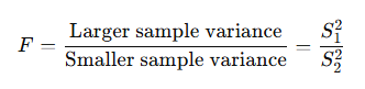
- ANOVA uses the F-statistic, which represents the ratio of variance between group means to the variance within the groups.
- Data Type Requirements
- Both tests require the dependent variable to be continuous.
- However, ANOVA is more scalable and better suited when analyzing data involving multiple groups.
- Error and Robustness
- As the number of comparisons increases, performing multiple T-tests raises the risk of Type I error.
- ANOVA controls this risk by analyzing all group differences simultaneously, making it more robust when dealing with more than two groups.
- Types of Tests
| Test Type |
Description |
| T-Test |
One-sample, two-sample (independent), paired sample |
| ANOVA |
One-way ANOVA (single factor), Two-way ANOVA (two factors with interaction) |
- Summary Comparison Table
| Criteria |
ANOVA |
T-Test |
| Meaning |
A statistical technique used to compare the means of 3 or more groups |
A statistical test to compare the means of 2 groups |
| Types |
One-way and Two-way ANOVA |
One-sample, two-sample, paired-sample t-tests |
| Focus |
Compares between-group and within-group variances |
Compares the mean difference between two groups |
| Population Size |
Can be applied to larger populations |
Best suited for smaller populations (n < 30) |
| Test Statistic |
F-value |
t-value |
| Interpretation |
High F-value suggests significant variance between group means |
High t-value suggests significant mean difference |
| Error Risk |
Slightly more risk due to multiple group comparisons |
Less error-prone, but limited to two-group comparisons |