Votre panier est actuellement vide !
Étiquette : mathematical-and-trigonometry-function
How to use the TANH() function in Excel
This function returns the hyperbolic tangent of a number.
Syntax
TANH(number)Argument
- number (required) – Any real number.
Background
- The hyperbolic tangent is part of the hyperbolic functions, which (like trigonometric functions) are defined for all real and complex numbers. However, Excel only supports real-number arguments for hyperbolic functions.
- The formula for the hyperbolic tangent is:
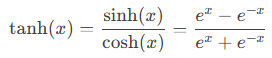
The last term highlights its similarity to trigonometric functions.
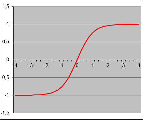
- The hyperbolic tangent is widely used in engineering and natural sciences for research and development (see Figure below).
Missing Cotangent Functions
- Unlike trigonometric functions (sin, cos, tan, cot), Excel does not include built-in hyperbolic cotangent (COTH) or trigonometric cotangent (COT) functions.
- However, both can be derived as reciprocals of their tangent counterparts:
- Trigonometric cotangent:
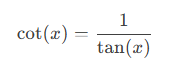
-
- Hyperbolic cotangent:
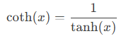
- Workaround in Excel:
Instead of =COTH(A1) (which does not exist), use:
=1/TANH(A1)
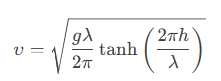
Example: Wave Propagation Speed Calculation
Application:
The hyperbolic tangent is used to calculate the propagation speed (υυ) of waves, given:- Gravity acceleration (gg) in [m/s²],
- Wave length (λλ) in [m],
- Water depth (hh) in [m].
Formula:
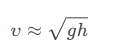
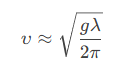
Approximations for Shallow/Deep Water:
- Shallow water (h≪λh≪λ):
- Deep water (h≫λh≫λ):
Additional Examples
=TANH(0) // Returns 0
=TANH(1) // Returns 0.761594156
=TANH(-1) // Returns -0.76159416
=TANH(10) // Returns 1 (approaches asymptotically)
=TANH(-10) // Returns -1 (approaches asymptotically)
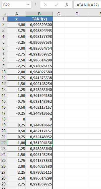
Key Properties:
- Output ranges between -1 and 1.
- For large positive/negative inputs, TANH() approaches ±1.
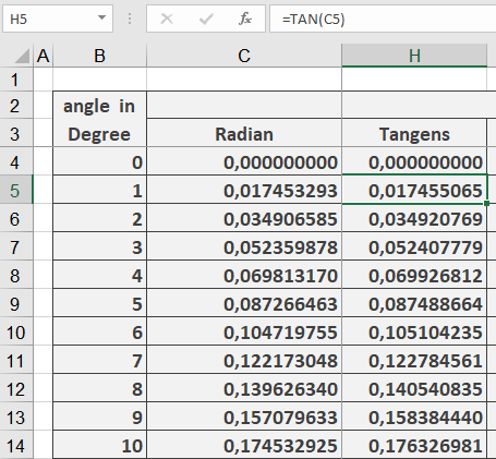
How to use the TAN() function in Excel
This function returns the tangent of an angle.
Syntax
TAN(number)Argument
- number (required) – The angle in radians for which you want the tangent.
Background
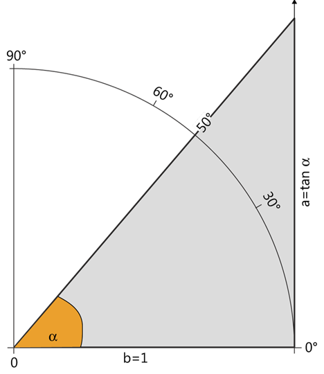
- In a right triangle, the tangent of an angle is the ratio of the length of the opposite side to the length of the adjacent side.
- The TAN() function requires the angle to be in radians. If the angle is given in degrees, convert it by multiplying by PI()/180 or using the RADIANS() function.
- For an angle α in a unit circle (r=1):
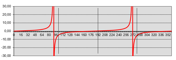
- As α increases from 0° to 90°, the tangent increases from 00 to +∞+∞ (see Figure below).
- In a coordinate system, plotting the angle αα on the x-axis and tan(α)tan(α) on the y-axis produces the curve shown in Figure below.
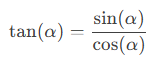
Tangent Relationship with Sine and Cosine:
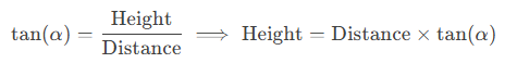
Practical Application (Slope Calculation):
- The tangent describes the relationship between the gradient angle and the slope of a line.
- Example: A road with a gradient angle of 12°12° has a slope of tan(12°)≈0.21tan(12°)≈0.21, often displayed as 21% (21 meters elevation per 100 meters horizontally).
- Note: The tangent is undefined at 90° and −90° (vertical slope).
Example:
Key Steps:
- Convert degrees to radians (RADIANS()).
- Calculate tangent (TAN()).
- Multiply by distance and round (ROUND()).
- Add observer’s eye level.
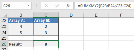
How to use the SUMXMY2() function in Excel
This function returns the sum of squares of differences of corresponding values in two arrays.
Syntax
SUMXMY2(array_x; array_y)Arguments
- array_x(required) – The first array or range of values.
- array_y(required) – The second array or range of values.
Background
- The arguments should be numbers, names, arrays, or references containing numbers.
- If an array or a reference argument contains text, logical values, or empty cells, those values are ignored. However, cells with the value zero are included.
- If array_xand array_y have a different number of values, the SUMXMY2() function returns the #N/A
The equation for the sum of squared differences is:
Σ(x – y)²The solution of this equation is built for the example (see Figure below) as follows:
- In two specified ranges:
- Range A:4, 5
- Range B:2, 3
The corresponding values are subtracted:
- First pair: 4 – 2 = 2
- Second pair: 5 – 3 = 2
- The differences are squared and summed (see Figure 16-37):
- 2² + 2² = 4 + 4 = 8
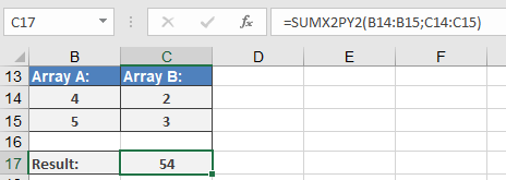
How to use the SUMX2PY2() function in Excel
This function returns the sum of the sum of squares of corresponding values in two arrays. The sum of the sum of squares is a common term in many statistical calculations.
Syntax
SUMX2PY2(array_x; array_y)Arguments
- array_x(required) – The first array or range of values.
- array_y(required) – The second array or range of values.
Background
- The arguments should be numbers, names, arrays, or references containing numbers.
- If an array or a reference argument contains text, logical values, or empty cells, those values are ignored. However, cells with the value zero are included.
- If array_xand array_y have a different number of values, the SUMX2PY2() function returns the #N/A
The equation for the sum of the sum of squares is:
Σ(x² + y²)EXAMPLE
The solution of this equation is built for the example (see Figure below) as follows:
- In two specified ranges:
- Range A:4, 5
- Range B:2, 3
The square of each value is calculated:
- Range A:16, 25
- Range B:4, 9
- The squares of all values in each range are summed:
- Range A:16 + 25 = 41
- Range B:4 + 9 = 13
- The sums are added together (see Figure 16-36):
41 + 13 = 54
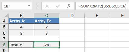
How to use the SUMX2MY2() function in Excel
This function returns the sum of the difference of squares of corresponding values in two arrays .
Syntax
SUMX2MY2(array_x; array_y)
Arguments
- array_x (required) – The first array or range of values.
- array_y (required) – The second array or range of values.
Background
- The arguments should be numbers or names, arrays, or references containing numbers.
- If an array or reference argument contains text, logical values, or empty cells, those values are ignored. However, cells with the value zero are included.
- If array_x and array_y have a different number of values, the SUMX2MY2() function returns the #N/A error.
The equation for the sum of the difference of squares is:
Σ(x² – y²)EXAMPLE
The solution for this equation is built for the example (see Figure below) as follows:
- In two specified ranges:
- Range A: 4, 5
- Range B: 2, 3
The square of each value is calculated:
-
- Range A: 16, 25
- Range B: 4, 9
- The squared values are summed:
- Range A: 16 + 25 = 41
- Range B: 4 + 9 = 13
- The sums are subtracted (see Figure below):
41 – 13 = 28
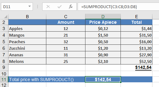
How to use the SUMPRODUCT() function in Excel
Its multiplies corresponding components in given arrays and returns the sum of those products.
Syntax:
SUMPRODUCT(array1; [array2]; [array3]; …)Arguments:
Argument Description array1 (required) First array of values array2 (required) Second array of values array3,… (optional) Additional arrays (up to 255 in modern Excel) Key Features:
- Calculation Method:
- Performs element-wise multiplication (a₁×b₁, a₂×b₂,…)
- Sums all resulting products
- Formula: Σ(array1[i] × array2[i] × …)
- Requirements:
- All arrays must have identical dimensions
- Non-numeric values are treated as zero
- Returns #VALUE! if arrays have different sizes
Example: Product Price Calculation
Common Errors:
- #VALUE!: Array size mismatch
- Incorrect results: Hidden text values treated as zero
Related Functions:
- SUM(): Simple addition
- MMULT(): Matrix multiplication
- SUMIFS(): Conditional sum with multiple criteria
Note:
While originally designed for simple array multiplication, SUMPRODUCT has become a powerful tool for complex array operations in Excel.- Calculation Method:
How to use the SUMIFS() function in Excel
Its adds all numbers in a range that meet multiple specified criteria (introduced in Excel).
Syntax:
SUMIFS(sum_range; criteria_range1; criteria1; [criteria_range2; criteria2]; …)Arguments:
Argument Description sum_range (required) Range of cells to sum criteria_range1 (required) First range to evaluate criteria1 (required) First condition (number, expression, or text) criteria_range2, criteria2,… (optional) Additional ranges/criteria (up to 127 pairs) Key Features:
- Criteria Formats:
- Number: 32
- Comparison: « >32 »
- Text: « apples » (exact) or « a* » (wildcard)
- Cell reference: I7
- Behavior:
- All criteria must be met for inclusion
- Case-insensitive text matching
- Supports wildcards (*, ?)
- More flexible than SUMIF() (which allows only 1 criterion)
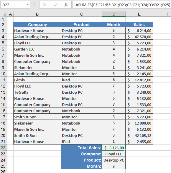
Example: Sales by Month, Company & Product
Scenario: Sum sales for « Contoso, Ltd. » purchasing « Desktop PC » in « Month 3 »Data Structure:
B3:B21 = Companies
C3:C21 = Products
D3:D21 = Months
E3:E21 = Sales amounts
I7 = « Contoso, Ltd. »
I8 = « Desktop PC »
I9 = 3 (Month)
Formula:
=SUMIFS(E3:E21; B3:B21; I7; C3:C21; I8; D3:D21; I9)
Breakdown:
- Sums values in E3:E21 where:
- B3:B21 matches « Contoso, Ltd. »
- C3:C21 matches « Desktop PC »
- D3:D21 equals 3
- Returns $5,723
Practical Notes:
- Order of criteria doesn’t affect results
- Ranges must be same size (but non-contiguous)
- For single-criterion sums, SUMIF() is simpler
Common Errors:
- #VALUE!: Mismatched range sizes
- Unexpected results: Verify criteria syntax (e.g., « > »&I9 for dynamic comparisons)
Related Functions:
- SUMIF(): Single-criterion version
- COUNTIFS(): Count with multiple criteria
- AVERAGEIFS(): Average with multiple criteria
- Criteria Formats:
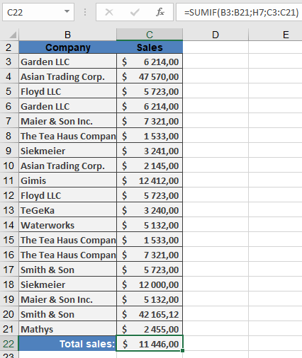
How to use the SUMIF() function in Excel
Its adds all values in a range that meet specified criteria.
Syntax:
SUMIF(range; criteria; [sum_range])Arguments:
Argument Description range (required) Range of cells to evaluate against the criteria criteria (required) Condition that determines which cells to add (number, expression, or text) sum_range (optional) Actual cells to sum (if omitted, uses ‘range’ for summing) Key Features:
- Criteria Formats:
- Number: 32
- Comparison: « >32 »
- Text: « apples » (exact match) or « a* » (wildcard match)
- Cell reference: A9
- Behavior:
- Case-insensitive for text criteria
- Supports wildcards (* for multiple characters, ? for single character)
- Omitting sum_range sums the criteria range itself
Example: Sales by Representative
Notes:
- For multiple criteria, use SUMIFS()
- Related functions:
- COUNTIF(): Count cells meeting criteria
- AVERAGEIF(): Average cells meeting criteria
Common Errors:
- #VALUE!: Incompatible criteria type
- Incorrect sums: Verify ranges are same size when using sum_range
- Criteria Formats:
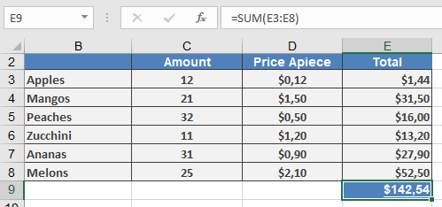
How to use the SUM() Function in Excel
Its returns the sum of all specified numbers or ranges.
Syntax:
SUM(number1; [number2]; …)Arguments:
Argument Description number1 Required. First number or range to sum number2,… Optional. Additional values to sum (1-254 total) Key Features:
- Input Flexibility:
- Accepts individual numbers (=SUM(1,2,3))
- Accepts cell ranges (=SUM(A1:A10))
- Accepts mixed arguments (=SUM(A1:A5,10,B2:B4))
- Automatic Handling:
- Ignores empty cells, text, and logical values in ranges
- Converts numeric text (« 12 ») to numbers
- Treats TRUE as 1 and FALSE as 0
- Returns errors if arguments contain error values
Technical Specifications:
- Maximum 255 arguments
- Works with numbers up to 15-digit precision
- Processes up to 32,767 characters in formula text
Examples:
Best Practices:
- Use the Alt+= shortcut for quick sum insertion
- For conditional sums, consider:
- SUMIF() for single criteria
- SUMIFS() for multiple criteria
- To sum only visible cells, use SUBTOTAL(9, range)
Common Errors:
Error Cause Solution #VALUE! Non-numeric text argument Verify data types #REF! Invalid reference Check range addresses #NAME? Misspelled function Correct to « SUM » Version Notes:
- Behavior consistent across all Excel versions
- Argument limit increased from 30 to 255 in Excel 2007
Related Functions:
- SUBTOTAL(): Ignore filtered/hidden rows
- SUMIF(): Conditional summation
- SUMPRODUCT(): Sum of products
- Input Flexibility:
How to use the SUBTOTAL() function in Excel
This function returns a subtotal for a range of data, typically used in lists or databases. While the Data > Subtotal command is often easier for creating subtotals, the SUBTOTAL() function allows for post-creation modifications.
Syntax:
SUBTOTAL(function_num; ref1; [ref2]; …)Arguments:
- function_num (required)
- A number between 1–11 (includes hidden rows) or 101–111 (excludes hidden rows) that specifies the calculation method.
Table 1: Function Codes
Code (Includes Hidden) Code (Excludes Hidden) Function 1 101 AVERAGE() 2 102 COUNT() 3 103 COUNTA() 4 104 MAX() 5 105 MIN() 6 106 PRODUCT() 7 107 STDEV() 8 108 STDEVP() 9 109 SUM() 10 110 VAR() 11 111 VARP() - ref1, ref2, …
- ref1 (required): The range to subtotal.
- ref2 (optional): Additional ranges (up to 254 total).
Key Features:
- Filters & Hidden Rows:
- Codes 1–11 include rows hidden manually (Format > Hide).
- Codes 101–111 exclude manually hidden rows.
- Always ignores rows filtered out (regardless of code).
- Nested Subtotals:
- Automatically skips other SUBTOTAL() results within the range to avoid double-counting.
- Limitations:
- Fails with 3D references (#VALUE! error).
- Designed for vertical ranges (columns). Hiding columns in horizontal ranges (e.g., =SUBTOTAL(109,B2:G2)) has no effect.
Example: Filtered Sum
Scenario: Calculate total sales for Michigan after filtering.
- Original Data (C2:C8):
=SUBTOTAL(9, C2:C8) // Sum all visible rows (includes hidden)
or
=SUBTOTAL(109, C2:C8) // Sum only non-hidden rows
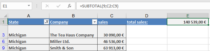
- After Filtering (Michigan):
- The result automatically updates to exclude filtered-out states.
Note: For dynamic reports, combine with Excel’s Filter or Table features.
- function_num (required)