Votre panier est actuellement vide !
Catégorie : Excel function
How to use the WORKDAY.INTL function in Excel
This advanced function calculates a date before or after a specified number of workdays, with customizable weekend days and optional holiday exclusions.
Syntax:
WORKDAY.INTL(start_date, days, [weekend], [holidays])Arguments:
- start_date (required): Beginning date for calculation (serial number or date text)
- days (required): Number of workdays to add (positive) or subtract (negative)
- weekend (optional): Defines non-working days using either:
- Predefined number codes (1-14)
- 7-character binary string (0=workday, 1=weekend)
- holidays (optional): Additional non-working dates to exclude
Background:
WORKDAY.INTL() extends WORKDAY() with customizable weekends. Key features:- Supports 14 predefined weekend patterns (Table 7-3)
- Allows custom weekend definitions via 7-digit binary strings
- Maintains all WORKDAY() functionality including holiday exclusion
- Ideal for international business with non-standard workweeks
Weekend Options:
Number Weekend Days String 1 Saturday-Sunday 0000011 2 Sunday-Monday 1000001 3 Monday-Tuesday 1100000 … … … 14 Saturday only 0000010 Important Notes:
- Defaults to Saturday-Sunday weekend (code 1) if omitted
- String must contain exactly seven 0/1 characters
- All-1 string (1111111) is invalid
- Returns #NUM! for invalid date results
- Returns #VALUE! for invalid inputs
- Truncates decimal day values
Examples:
- Standard workweek:
=WORKDAY.INTL(TODAY(), 14) → 14 business days from today (Sat/Sun off) - Middle Eastern workweek (Fri/Sat off):
=WORKDAY.INTL(« 01/01/2023 », 10, 7) → 10 workdays (Fri/Sat weekends) - Custom 4-day workweek (Wed/Thu/Fri off):
=WORKDAY.INTL(« 06/01/2023 », 15, « 0011100 ») - With holidays:
=WORKDAY.INTL(« 12/12/2022 », 10, 1, {« 12/25/2022″, »12/26/2022 »})

Formatting:
- Holiday lists must use curly braces: {« date1″, »date2 »}
- Date strings should match system locale settings
- For readability, consider using cell references for holiday lists
How to use the WORKDAY function in Excel
This function calculates the date that is a specified number of workdays before or after a start date, excluding weekends and optional holidays.
Syntax:
WORKDAY(start_date, days, [holidays])Arguments:
- start_date (required): The beginning date for the calculation
- days (required): Number of workdays to add (positive) or subtract (negative)
- holidays (optional): List of dates to exclude as non-working days (e.g., public holidays)
Background:
Use WORKDAY() to:- Calculate payment due dates based on business days
- Determine project deadlines excluding weekends/holidays
- Schedule deliveries within working days
Key features:
- Excludes Saturdays/Sundays by default
- Doesn’t count the start_date in calculations
- Holidays can be specified as a range or array constant
- Unlike NETWORKDAYS(), doesn’t include start date in count
Important notes:
- Returns #VALUE! for invalid dates
- Returns #NUM! if result is outside valid date range
- Truncates decimal values in days argument
Examples:
- Basic calculation:
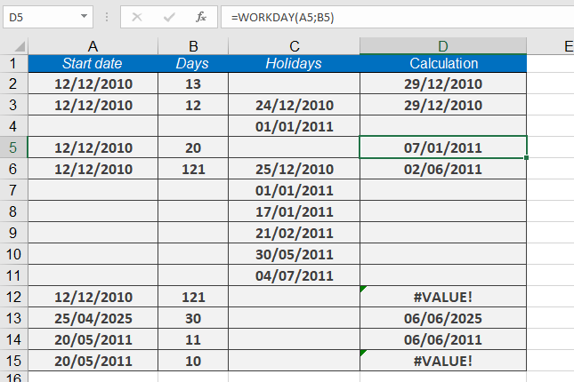
=WORKDAY(TODAY(), 30) → Returns date 30 workdays from today - With holiday exclusion:
=WORKDAY(« 12/12/2010 », 12, {« 12/24/2010″, »01/01/2011 »}) → Returns 12/29/2010 - Negative days:
=WORKDAY(« 01/15/2023 », -10) → Returns date 10 workdays before Jan 15, 2023
Formatting Note:
When entering holidays directly in formula, use curly braces {} not parentheses.How to use the WEEKNUM function in Excel
This function returns the week number (as an integer) for a given date.
Syntax:
WEEKNUM(serial_number, [return_type])Arguments:
- serial_number (required): The date for which to calculate the week number.
- return_type (optional): A number specifying the week numbering system and starting day.
Options in Excel :
-
- 1 (System 1, default): Week begins on Sunday (days numbered 1–7, Sunday=1).
- 2 (System 2): Week begins on Monday (days numbered 1–7, Monday=1).
Additional options in Excel :
-
- 1: Week begins on Sunday (default).
- 2: Week begins on Monday.
- 11: Week begins on Monday.
- 12: Week begins on Tuesday.
- 13: Week begins on Wednesday.
- 14: Week begins on Thursday.
- 15: Week begins on Friday.
- 16: Week begins on Saturday.
- 17: Week begins on Sunday.
- 21 (System 2, ISO 8601): Week begins on Monday.
Background:
- System 1: Week 1 is the week containing January 1.
- System 2 (ISO 8601): Week 1 is the week with the year’s first Thursday (European standard).
- System 2 aligns with ISO 8601 (1988), where weeks start on Monday.
Example:
How to display week numbers in an operations schedule:
=WEEKNUM(date)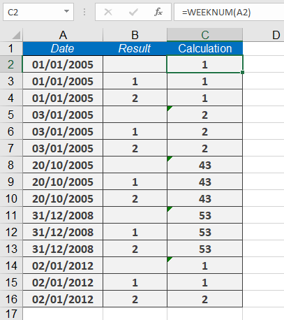
How to use the WEEKDAY function in Excel
This function converts a date (serial number) into a weekday number, returning an integer from 1 (Sunday) to 7 (Saturday) by default.
Syntax:
WEEKDAY(serial_number, [return_type])Arguments:
- serial_number (required): The date for which to calculate the weekday number.
- return_type (optional): A number (1, 2, or 3) that determines the numbering system for weekdays:
- 1 (or omitted): 1 = Sunday, 2 = Monday, …, 7 = Saturday (default).
- 2: 1 = Monday, 2 = Tuesday, …, 7 = Sunday.
- 3: 0 = Monday, 1 = Tuesday, …, 6 = Sunday.
additional return types are available:
-
- 11: 1 = Monday, 2 = Tuesday, …, 7 = Sunday.
- 12: 1 = Tuesday, 2 = Wednesday, …, 7 = Monday.
- 13: 1 = Wednesday, 2 = Thursday, …, 7 = Tuesday.
- 14: 1 = Thursday, 2 = Friday, …, 7 = Wednesday.
- 15: 1 = Friday, 2 = Saturday, …, 7 = Thursday.
- 16: 1 = Saturday, 2 = Sunday, …, 7 = Friday.
- 17: 1 = Sunday, 2 = Monday, …, 7 = Saturday.
Background:
Use WEEKDAY() to extract the day of the week from a date. As an alternative, the TEXT() function can return the weekday as a text string (e.g., =TEXT(TODAY(), « dddd »)).Example:
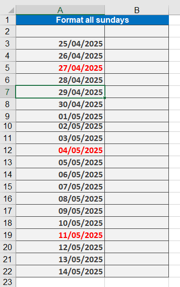
To highlight Sundays in red within a date column:- Select the date column.
- Apply conditional formatting:
- Go to Format > Conditional Formatting, select Formula, and enter:
=WEEKDAY(A1, 1) = 1
- Go to Format > Conditional Formatting, select Formula, and enter:
OR
- Click Conditional Formatting > New Rule > « Use a formula », then enter the formula above.
- Set the formatting to red.
Enter the formula
=WEEKDAY($B11,1)=1
and click the Format button to format the text
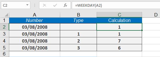
The following examples show how the type parameter works:
=WEEKDAY(« 08/03/2008 »,1) returns 1 (Sunday).
=WEEKDAY(« 08/03/2008 »,2) returns 7.
=WEEKDAY(« 08/03/2008 »,3) returns 6.
How to use the TODAY function in Excel
This function returns the serial number corresponding to the current date.
Syntax:
TODAY()Background:
The TODAY() function retrieves the current date without including the time. If the cell is formatted as General before entering the function, the result will display as a date.The related NOW() function returns both the current date and time, whereas TODAY() provides only the date.
Use TODAY() to calculate date differences from the current date. For example, you can determine how many days have passed since an invoice was issued, helping track deadlines.
Results update when:
- The workbook is opened
- A manual recalculation is triggered (press F9 to refresh)
Note: The function’s accuracy relies on your system’s correct date and time settings.
Example:
To insert the current date in an invoice form, use:
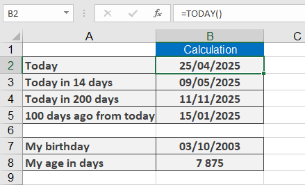
=TODAY()Additional examples:
- =TODAY()+14 → Returns the date 14 days from today.
- =TODAY()+200 → Returns the date 200 days from today.
- =TODAY()-100 → Returns the date 100 days before today.
- =TODAY()-« 11/14/1959 » → Calculates a person’s age in days if their birthdate is November 14, 1959.
How to use the TIMEVALUE function in Excel
This function converts a time formatted as text into a time value (serial number). The serial number is a value in the range of 0 through 0.99999999, corresponding to a time from 00:00:00 through 23:59:59.
Syntax:
TIMEVALUE(time_text)Arguments:
- Time_text (required): A text value in any Excel time format. Dates in the time argument are ignored.
Background:
If a time is formatted as text (e.g., in imported values), use the TIMEVALUE() function to convert it into a serial number. The result can then be used in other calculations.Most Excel functions automatically convert text-formatted times into serial numbers. However, with imported data or third-party add-in functions, this may not always happen. To ensure proper conversion, use TIMEVALUE().
Example:
Assume that after importing data, some values appear as text in a time column. To use them in calculations, convert them into numeric time values.The formula:
=TIMEVALUE(« 06:00:00 »)
returns the time value 0.25 (or 06:00 when formatted as hh:mm). This is a valid time value in Excel’s time system.Additional examples:
- =TIMEVALUE(« 06:00 PM ») returns 0.75.
- =TIMEVALUE(« 06:45:16 ») returns 0.281435185.
- =TIMEVALUE(« 12:00:00 ») returns 0.5.

How to use the TIME function in Excel
This function returns the serial number (decimal value) representing a time specified by the hour, minute, and second arguments.
Syntax: TIME(hour, minute, second)
Arguments:
- hour (required) – A number from 0 to 32,767 representing the hour.
- Values > 23 are divided by 24, and the remainder is used as the hour.
- Example: TIME(28,0,0) → TIME(4,0,0) (4:00 AM or 0.16667).
- minute (required) – A number from 0 to 32,767 representing the minute.
- Values > 59 are converted into hours and minutes.
- Example: TIME(0,150,0) → TIME(2,30,0) (2:30 AM or 0.1041667).
- second (required) – A number from 0 to 32,767 representing the second.
- Values > 59 are converted into hours, minutes, and seconds.
- Example: TIME(0,0,12011) → TIME(3,20,11) (3:20:11 AM or 0.139016204).
Background:
- When performing time calculations, you may need to break down a time into components (hours, minutes, seconds) and then reconstruct it.
- The TIME() function converts these parts back into a numeric time value (decimal between 0 and 0.99999999, representing 00:00:00 to 23:59:59).
- If the cell format is set to General before entering the function, the result displays as a time.
Examples:
For applications that include standard processing times in hours, minutes, and seconds, you might want to combine these to display a time value. To do this, use the formula
=TIME(standard_hours,standard_minutes,standard_seconds)
The following examples show possible results and exceptions if the 24- hour, 60-minute, or 60-second boundary is exceeded:
- Basic time construction:
- =TIME(5,6,11) → 05:06:11
- =TIME(13,10,0) → 13:10:00
- =TIME(23,45,30) → 23:45:30
- Handling overflow (values exceeding standard limits):
- =TIME(24,15,30) → 00:15:30 (24 hours wraps to 0)
- =TIME(26,30,30) → 02:30:30 *(26 – 24 = 2 hours)*
- =TIME(12,80,10) → 13:20:10 *(80 minutes = 1 hour + 20 minutes)*
- =TIME(12,59,120) → 13:01:00 *(120 seconds = 2 minutes)*

- hour (required) – A number from 0 to 32,767 representing the hour.
How to use the SECOND function in Excel
This function extracts the seconds from a serial number (a time value, with or without a date). The returned value is an integer between 0 and 59.
Syntax: SECOND(serial_number)
Arguments:
- serial_number (required) – A valid time (or a date-time value).
Background
Like the HOUR() and MINUTE() functions, SECOND() allows you to extract a component of a time value for use in calculations.
Times can be entered in different formats:
- As a text string in quotation marks (e.g., « 06:43:12 »),
- As a decimal number (e.g., 0.27986111 for 06:43),
- Or as the result of other formulas or functions (e.g., NOW()).
Examples:
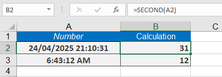
The following are examples where the function SECOND() extracts seconds from a date/time value:
- =SECOND(« 07/13/2008 20:48:31 ») → Returns 31.
- =SECOND(« 06:43:12 ») → Returns 12.
- =SECOND(NOW()) → Returns the current second.
How to use the NETWORKDAYS.INTL function in Excel
It is use to calculates the number of working days between two dates while excluding:
- Custom-defined weekends (not limited to Saturday/Sunday)
- Specified holidays
Syntax
NETWORKDAYS.INTL(start_date, end_date, [weekend], [holidays])
Arguments
- start_date (required): First day of the period.
- end_date (required): Last day of the period.
- weekend (optional): Defines non-working days. Options:
- Number codes (1-7, 11-17): Predefined weekend combinations (see table below).
- 7-digit string: Custom weekly off-days (e.g., « 0000011 » = Saturday/Sunday).
- Default: 1 (Saturday/Sunday off).
- holidays (optional): Additional non-working dates (cell range or array).
Weekend Codes Reference
Number Weekend Days String Equivalent 1 (default) Saturday, Sunday « 0000011 » 2 Sunday, Monday « 1000001 » 3 Monday, Tuesday « 1100000 » 4 Tuesday, Wednesday « 0110000 » 5 Wednesday, Thursday « 0011000 » 6 Thursday, Friday « 0001100 » 7 Friday, Saturday « 0000110 » 11 Sunday only « 0000001 » 12 Monday only « 1000000 » … … … 17 Saturday only « 0000010 » Note: Strings use 1 for off-days and 0 for workdays (e.g., « 0101000 » = Monday/Wednesday off).
Example
Assume that a project is planned from December 12, 2008, through June 2, 2009. You have to calculate the number of workdays in this timeframe, excluding holidays. The formula
=NETWORKDAYS.INTL(« 12/12/10″, »06/02/11 »,1,
{« 12/25/10″, »01/01/11″, »01/17/11 », »02/21/11 « , »05/30/2011″, »07/04/11 »})
returns 121 workdays for the project. Note that in the formula, holidays are enclosed in braces and not in parentheses.

Notes
- Error Handling: Returns #VALUE! for invalid dates or text entries.
- Flexibility: Supports any weekend pattern except « 1111111 » (no workdays).
- Pro Tip: Name your holiday range (e.g., Holidays) for cleaner formulas.
How to use the NETWORKDAYS function in Excel
The NETWORKDAYS function is use to calculates the number of working days between two dates, automatically excluding:
- Weekends (Saturday & Sunday)
- Custom holidays (if specified)
Syntax
NETWORKDAYS(start_date, end_date, [holidays])
Arguments
- start_date (required): First day of the period.
- end_date (required): Last day of the period.
- holidays (optional):
- A range of cells containing holiday dates
- An array of serial numbers (e.g., {« 1/1/2023 », « 12/25/2023 »})
Example
Assume that a project is planned to extend over the period from December 12, 2008, through June 2, 2009. You have to calculate the number of workdays in this timeframe, excluding holidays. The formula
=NETWORKDAYS(« 12/12/10″, »06/02/11 »,
{« 12/25/10″, »01/01/11″, »01/17/11″, »02/21/11 », « 05/30/2011″, »07/04/11 »})
returns 121 workdays for the project. Note that in the preceding formula, holidays are enclosed in braces and not in parentheses. The table below shows the calculation using cell references for the start date, end date, and holidays.

Key Features
- Inclusive Counting: Both start_date and end_date are counted if they are workdays.
- Holiday Handling: Excludes dates listed in the holidays argument.
- Error Cases: Returns #VALUE! for invalid dates or text entries.
Notes
- Alternative: Use NETWORKDAYS.INTL() for custom weekends (e.g., Friday-Saturday weekends).
- Tip: Name your holiday range (e.g., Holidays) for easier reference.
- Error Handling:
=IFERROR(NETWORKDAYS(Start, End, Holidays), « Check dates »)