Catégorie : Excel function

Its extracts the month number (1-12) from a date, where:

• 1 = January
• 12 = December

Syntax

MONTH(serial_number)

Arguments

• serial_number (required):
  • A valid date
  • Can be:
    • A date string (e.g., « 11/14/1959 »)
    • A serial number (Excel date format)
    • A cell reference containing a date
    • The result of another function (e.g., TODAY())

Background

Part of Excel’s date function family (with YEAR() and DAY()). Used to:

• Extract months for grouping/sorting data
• Support monthly reporting
• Enable date-based calculations

Examples

 Assume that you want to enable the Excel AutoFilter for the months and need to calculate the month values from a date column by using an auxiliary column. To do this, use the formula

=MONTH(date_value)

Here are more examples:

Formula	Returns	Explanation
=MONTH(TODAY())	9 (if current month is September)	Current month number
=MONTH(« 11/14/1959 »)	11	November extraction
=MONTH(« 01/01/1900 »)	1	January extraction
=MONTH(« 12/31/1899 »)	#VALUE!	Invalid date (pre-1900 in Windows)
=MONTH(« 12/31/9999 »)	#VALUE!	Invalid
=MONTH(« 01/01/10000 »)	#VALUE!	Invalid date (post-9999)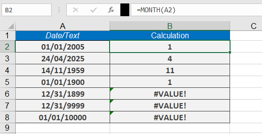

Notes

• Returns #VALUE! for:
  • Text-formatted dates
  • Dates outside Excel’s valid range (1/1/1900–12/31/9999 for Windows)
• Combine with YEAR() and DAY() for complete date analysis

The MINUTE function is use to extracts the minute component from a time value (with or without an associated date). Returns an integer between 0 and 59.

Syntax

MINUTE(serial_number)

Arguments

• serial_number (required):
  • A valid time value
  • Can be entered as:
    • A time string in quotes (e.g., « 06:43 »)
    • A decimal number representing time (e.g., 0.27986111 for 06:43)
    • The result of another formula/function (e.g., NOW())
    • A cell reference containing a time/date

Background

Part of Excel’s time function family (along with HOUR() and SECOND()). Used to:

• Extract minute values for time-based calculations
• Analyze scheduling data
• Build dynamic time-dependent formulas

Example

 Assume that you need to calculate the minutes after the full hours.

Here are example formulas:

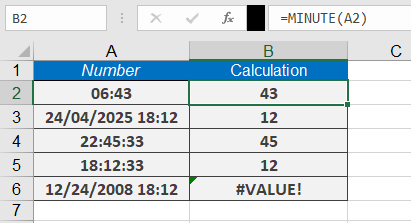
=MINUTE(« 06:43 ») returns 43 minutes.

=MINUTE(« 12/24/2010 18:12 ») returns 12.

=MINUTE(NOW()) returns the current minute.

Notes

• Returns #VALUE! for invalid time formats
• For decimal inputs:
  • 0.0 = 12:00:00 AM
  • 0.5 = 12:00:00 PM
  • 0.999 = 11:59:59 PM
• Combine with HOUR() and SECOND() for complete time extraction

This function is essential for time tracking, scheduling, and data analysis in Excel.

Its extracts the hour component from a time value (with or without an associated date). Returns an integer between 0 (midnight) and 23 (11 PM).

Syntax

HOUR(serial_number)

Arguments

• serial_number (required):
  • A valid time value
  • Can be entered as:
    • Time string in quotes (e.g., « 06:43 »)
    • Decimal number representing time (e.g., 0.27986111 for 06:43)
    • Result of other formulas/functions
    • Cell reference containing time/date

Background

Part of Excel’s time function family (along with MINUTE() and SECOND()). Used to:

• Extract hour components for calculations
• Analyze time-based data
• Create time-dependent formulas

Example

If you want to extract the hours from a time value, you can use the formula

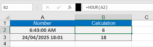
=HOUR(« 06:43 »)

which returns 6 hours.

Here are some more examples:

=HOUR(« 24/04/2025 18:01 ») returns 18.

=HOUR(NOW()) returns the current hour.

Notes

• Returns #VALUE! for invalid time formats
• For decimal inputs:
  • 0.0 = 12:00 AM
  • 0.5 = 12:00 PM
  • 0.999 = 11:59 PM
• Combine with MINUTE() and SECOND() for complete time breakdown

Its returns the serial number representing the last day of the month, calculated as a specified number of months before or after a given start date;

Syntax

EOMONTH(start_date, months)

Arguments

• start_date (required):
  • The initial date for calculation
  • Can be a date string, serial number, or reference to a cell containing a date
• months (required):
  • Integer value specifying the number of months to add (positive) or subtract (negative)
  • Decimal values are truncated (e.g., 2.9 becomes 2)

Background

Primarily used in financial applications for:

• Calculating payment due dates
• Determining maturity dates
• Setting month-end reporting periods

Alternative Calculation Method:

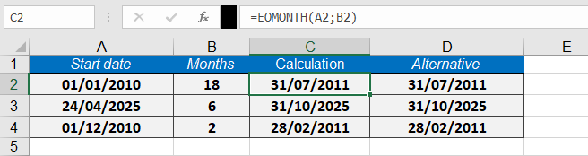
=DATE(YEAR(start_date), MONTH(start_date) + months + 1, 1) – 1

This formula:

1. Advances to the first day of the month after the target month
2. Subtracts one day to get the last day of the target month

Error Handling

• Returns #NUM! error if:
  • start_date is invalid or text-formatted
  • Resulting date falls outside Excel’s valid date range (1/1/1900 to 12/31/9999 for Windows)

Examples

Assume that you want to designate the last day of the month as the due date for a credit period 18 months from January 1, 2010. The formula

=EOMONTH(« 01/01/2010 »,18)

returns 07/31/2011 as the due date as seen bellow

This function is particularly valuable for financial professionals who need to calculate precise month-end dates for various accounting and reporting purposes.

The EDATE function is use to Returns the serial number of the date that is a specified number of months before or after a given start date.

Syntax

EDATE(start_date, months)

Arguments

• start_date (required): The initial date for the calculation.
• months (required): The number of months to add (positive) or subtract (negative).

Background

• Calculates future or past dates by adding/subtracting months while preserving the day value (unless invalid for the new month).
• Alternative method using DATE(), YEAR(), MONTH(), and DAY():

=DATE(YEAR(start_date), MONTH(start_date) + months, DAY(start_date)) 

• Errors:
  • #VALUE! if start_date is invalid.
  • Non-integer months are truncated (e.g., 3.9 becomes 3).

Examples

 Assume that you want to calculate the end of months of 4 construction project. The formula given bellow;

Formula	Result	Notes
=EDATE(« 01/02/2010 », 18)	07/02/2011	18 months later
=EDATE(« 01/02/2010 », 24)	01/02/2012	2 years later (24 months)
=EDATE(« 01/03/2010 », 0)	01/03/2010	Same date (months=0)
=EDATE(« 01/04/2010 », -5)	08/04/2009	5 months earlier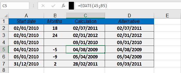

Key Notes

• Day Adjustment: If the resulting month has fewer days (e.g., =EDATE(« 31/01/2023 », 1)), Excel returns the last valid day (February 28 or 29).
• Formatting: Apply date formatting to display the serial number as a readable date.

The DAYS360 is use to calculates the number of days between two dates based on a 360-day year (12 months × 30 days each), commonly used in financial and accounting calculations.

Syntax

DAYS360(start_date, end_date, [method])

Arguments

• start_date (required): The beginning date of the period.
• end_date (required): The ending date of the period.
• method (optional): Specifies the calculation method:
  • FALSE or omitted: U.S. (NASD) method
    • If the start date is the last day of a month, it is treated as the 30th of the same month.
    • If the end date is the last day of a month:
      • If the start date is before the 30th, the end date becomes the 1st of the next month.
      • Otherwise, the end date becomes the 30th of the same month.
  • TRUE: European method
    • Any 31st of a month is treated as the 30th of the same month.

Background

• Primarily used for interest calculations in financial applications (e.g., bonds, loans).
• Returns a negative number if start_date > end_date.
• Always use the Excel percent format for interest rates (e.g., 5.25%).

Interest Calculation Formula

To compute interest over a period:

Interest = Capital × Interest Rate × DAYS360(start_date, end_date, [method]) / 360

Use ROUND() to format the result to 2 decimal places (currency format).

Example

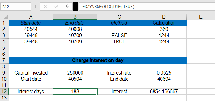
Calculate interest for $250,000 at 5.25% from November 22, 2010 (cell C12) to May 31, 2011 (cell E12):

1. Calculate Days (European method):

=DAYS360(C12, E12, TRUE) 

Returns: 188 days.

1. Compute Interest:

=C11 * E11 * DAYS360(C12, E12, TRUE) / 360 

Returns: $6,854.17.

Key Notes

• Error Handling: Ensure dates are valid (use IFERROR for robustness).
• Method Selection: Choose TRUE (European) or FALSE (U.S.) based on financial standards.

The DAY function extracts and returns the day number (1-31) from a given date.

Syntax

DAY(serial_number)

Arguments

• serial_number (required): The date value from which to extract the day. Can be:
  • A cell reference containing a date
  • A date serial number
  • A date entered as text in Excel-recognized format

Background

• Part of Excel’s date function family (along with YEAR() and MONTH())
• Extracts the day component for use in calculations or data analysis
• Works with Gregorian calendar dates only
• Returns #VALUE! error for invalid dates

Key Points

1. Date Systems:
   • Windows (1900 system): Valid dates 1/1/1900 to 12/31/9999
   • Mac (1904 system): Valid dates 1/1/1904 to 12/31/9999
2. Error Conditions:
   • Dates outside valid range return #VALUE!
   • Text that can’t be interpreted as a date returns #VALUE!
3. Practical Applications:
   • Extracting days for filtering or grouping
   • Date-based calculations
   • Data validation

Examples

Formula	Result	Notes
=DAY(« 07/13/2008 »)	13	Standard date format
=DAY(« 11/14/1959 »)	14	Day extraction
=DAY(« 01/01/1900 »)	1	Earliest valid date in Windows system
=DAY(« 12/31/1899 »)	#VALUE!	Before valid date range
=DAY(« 12/31/9999 »)	31	Latest valid date
=DAY(« 01/01/10000 »)	#VALUE!	Beyond valid date range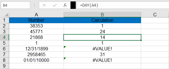

Note: For error handling with potentially invalid dates:

=IFERROR(DAY(A2), »Invalid Date »)

Converts a date stored as text into a serial number that Excel recognizes as a date.

Syntax

DATEVALUE(date_text)

Arguments

• date_text (required): A text string representing a date in any valid Excel date format.

Background

• Essential for converting imported or text-formatted dates into numeric values for calculations.
• While Excel often auto-converts text dates, DATEVALUE() ensures reliability with:
  • Imported data
  • Third-party add-in outputs
  • Non-standard date formats

Key Features

1. Date Systems:
   • Windows (1900 system): Accepts dates from 1/1/1900 to 12/31/9999
   • Mac (1904 system): Accepts dates from 1/1/1904 to 12/31/9999
   • Out-of-range dates: Return #VALUE! error
2. Partial Dates:
   • Missing year: Uses current system year
   • Missing day: Defaults to 1st of month
   • Time values: Always ignored
3. Format Flexibility:
   • Supports multiple text date formats (MM/DD/YYYY, DD-MM-YYYY, Month YYYY, etc.)

Examples

Formula	Result (Windows)	Notes
=DATEVALUE(« 12/12/2008 »)	39794 (displays as 12/12/2008)	Full date conversion
=DATEVALUE(« 11/11 »)	11/11/[current year]	Auto-fills current year
=DATEVALUE(« August 2007 »)	08/01/2007	Month-year becomes 1st of month
=DATEVALUE(« 2008/11/22 »)	11/22/2008	Handles YYYY/MM/DD format

as shown below;

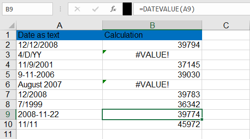
Note: Combine with error checking for imported data:

=IFERROR(DATEVALUE(A2), « Invalid Date »)

This function calculates the time interval (period) between a start date and an end date, returning the result in years, months, or days based on the specified unit.

Syntax

DATEDIF(start_date, end_date, unit)

Arguments

• start_date (required) – The beginning date of the period.
• end_date (required) – The ending date of the period.
• unit (required) – The type of interval to calculate. Available options:
  • « Y » → Full years in the period.
  • « M » → Full months in the period.
  • « D » → Total days in the period.
  • « MD » → Days remaining after whole months (ignores months and years).
  • « YM » → Months remaining after whole years (ignores years and days).
  • « YD » → Days remaining as if dates were in the same year (ignores years).

Background

DATEDIF() computes the difference between two dates, which can be entered as:

• Text strings (e.g., « 01/01/2020 »),
• Serial numbers (Excel’s date format), or
• Results of other formulas/functions (e.g., TODAY()).

Examples

1. Calculating Employment Duration (Years):

=DATEDIF(« 01/01/2006 », « 11/13/2011 », « Y ») 

Result: 5 (years from January 1, 2006, to November 13, 2011).

2. Calculating Employment Duration (Months):

=DATEDIF(« 01/01/2006 », « 11/30/2011 », « M ») 

Result: 70 (full months between the dates).

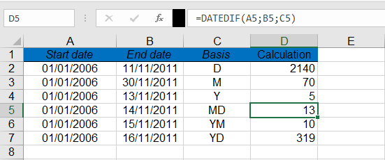
Note:

• « MD », « YM », and « YD » units exclude higher time units (e.g., « MD » only compares days).
• Ensure end_date is later than start_date to avoid errors.

 

This function returns the serial number representing a date based on the specified year, month, and day arguments.

Syntax

DATE(year, month, day)

Arguments

• year (required) – The year value (1 to 4 digits). Recommended: Use 4 digits.
• month (required) – A numeric value for the month (1 to 12).
• day (required) – A numeric value for the day (1 to 31).

Background

When working with date calculations, you may need to combine separate year, month, and day values into a single date. The DATE() function converts these components into a numeric date format that Excel can use in further calculations.

Excel interprets the year argument based on your system’s date settings:

• Windows (1900 Date System)
  • Years 0–1899: Excel adds the value to 1900 (e.g., DATE(99,1,1) = January 1, 1999).
  • Years 1900–9999: Excel uses the exact value (e.g., DATE(2023,5,10) = May 10, 2023).
  • Invalid years (negative or ≥ 10,000) return #NUM!.
• Mac (1904 Date System)
  • Years 4–1899: Excel adds the value to 1900 (e.g., DATE(50,1,1) = January 1, 1950).
  • Years 1904–9999: Excel uses the exact value (e.g., DATE(2025,12,25) = December 25, 2025).
  • Invalid years (< 4, ≥ 10,000, or 1900–1903) return #NUM!.

Handling Month & Day Overflow

• If month > 12, Excel adds the excess months to the first month of the given year.
  • Example: DATE(2023,14,1) = February 1, 2024 (14 – 12 = 2 months into the next year).
• If day exceeds the month’s days, Excel adds the excess days to the first day of the month.
  • Example: DATE(2023,1,35) = February 4, 2023 (35 – 31 = 4 days into the next month).

Examples

Calculating the First and Last Day of a Month

In accounting applications, you may need to determine the first and last day of a month for a given date.

• First day of the month:

=DATE(YEAR(« 07/23/2008 »), MONTH(« 07/23/2008 »), 1) 

Result: 07/01/2008
Explanation: The formula extracts the year and month from the given date (07/23/2008) and sets the day to 1, returning the first day of the month.

• Last day of the month:

=DATE(YEAR(« 07/23/2008 »), MONTH(« 07/23/2008 ») + 1, 1) – 1 

Result: 07/31/2008
Explanation:

• • The formula calculates the first day of the next month (by adding +1 to the month).
  • Subtracting 1 day gives the last day of the original month.

Additional Examples

1. Two-digit year (1900 date system):

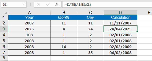
=DATE(108, 1, 2) 

Result: 01/02/2008
Explanation: Excel adds 108 to 1900, resulting in 2008.

2. Four-digit year:

=DATE(2008, 1, 2) 

Result: 01/02/2008

3. Month overflow (greater than 12):

=DATE(2008, 14, 2) 

Result: 02/02/2009
Explanation: Since 14 exceeds 12, Excel adds 2 months to January 2008, rolling into February 2009.

4. Day overflow (greater than days in the month):

=DATE(2008, 1, 35) 

Result: 02/04/2008
Explanation: January has 31 days, so 35 – 31 = 4, resulting in February 4, 2008.