Votre panier est actuellement vide !
Catégorie : Excel function
How to use the LEN and LENB function in Excel
The LEN() function returns the number of characters in a string. The LENB() function returns the number of bytes used by double-byte characters in a string.
Syntax
LEN(text)
LENB(text)Arguments
- text(required): The text for which you want to determine the length.
Background
This function is useful for various tasks, such as combining it with other functions like MID(), LEFT(), or RIGHT() to manipulate strings.You can use LEN() to verify whether an entry meets a specific length requirement or to check if text in a column exceeds a defined limit. The function counts spaces and numerals as characters.
Example
Suppose you need to ensure that interface descriptions in a column do not exceed 10 characters. You can use LEN() along with AutoFilter to quickly identify and correct strings longer than 10 characters.Additional examples:
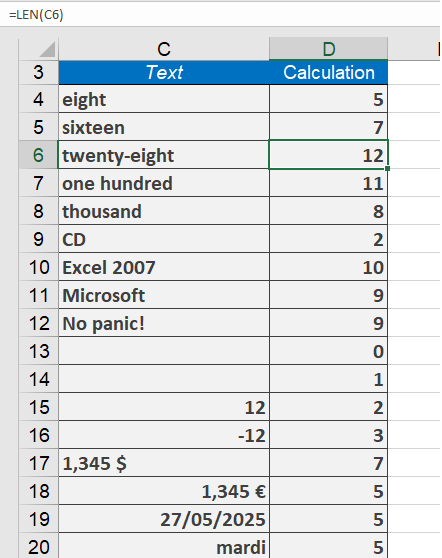
- =LEN(« CD »)returns 2.
- =LEN(« Excel 2007 »)returns 10.
- =LEN(« Microsoft »)returns 9.
- =LEN(« No Panic! »)returns 9.
- =LEN(« »)returns 0.
- =LEN( » « )returns 1.
- =LEN(« 1.345 $ »)returns 7.
- =LEN(TODAY())returns 5.
How to use the LEFT and LEFTB function in Excel
The LEFT function returns the first characters of a string. The LEFTB function is used for double-byte characters and returns the first bytes.
Syntax
LEFT(text; num_chars)
LEFTB(text; num_bytes)Arguments
- text(required): The string containing the characters you want to extract.
- num_chars/num_bytes(optional): Specifies how many characters/bytes to extract.
Background
Use the LEFT function to extract the first part of a string. You can enter letters or numbers in the text argument. The functions LEFT, RIGHT, and MID are especially useful if strings follow a specific pattern, such as ZIP codes, locations, or ISBNs.The num_chars argument must be greater than or equal to 0. If num_chars exceeds the length of the text argument, LEFT() returns the entire string. If num_chars is omitted, the default value is 1.
Example
A list of names is entered into a spreadsheet column, with the first name separated from the last name by a space. Cell H4 contains a name.The following formula extracts the first name:
=LEFT(H4; SEARCH( » « ; H4) – 1)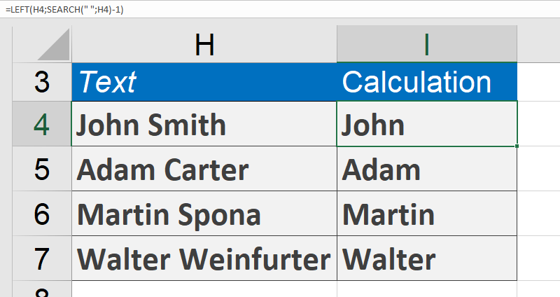
The SEARCH function determines the position of the space between the first and last names. Subtracting 1 gives the position of the last character of the first name (the number of characters from the left).
Additional Examples
- =LEFT(« steamboat »; 5)returns steam.
- =LEFT(« gazelle »; 4)returns gaze.
- =LEFT(« Oliver Kiel »; 5)returns Oliver.
- =LEFT(« Excel »; 1)returns E.
- =LEFT(« Excel »; 2)returns Ex.
Creating Dates and Highlighting Weekdays in Excel VBA
The function DateSerial() is used to create a date, while the function Weekday() determines the day of the week for a given date. Below, these two functions are used to highlight weekend days specifically:
Sub HighlightWeekend()
    Dim i As Integer
    Dim currentDate As Date
    ThisWorkbook.Worksheets("Sheet1").Activate
    For i = 1 To 31
        currentDate = DateSerial(2025, 1, i)   ' Create a date for January 2025
        Cells(i, 7).Value = currentDate         ' Put the date in column G (7th column)
        Cells(i, 7).NumberFormat = "ddd. dd.mm.yy" ' Format the date display
        If Weekday(currentDate, vbSunday) = 7 Then
            Cells(i, 7).Interior.Color = vbYellow  ' Highlight Saturdays in yellow
        ElseIf Weekday(currentDate, vbSunday) = 1 Then
            Cells(i, 7).Interior.Color = vbGreen   ' Highlight Sundays in green
        Else
            Cells(i, 7).Interior.Pattern = xlNone   ' No fill for weekdays
        End If
    Next i
End Sub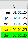
Explanation:
All dates of January 2020 are listed vertically. A loop runs from 1 to 31 to generate each day.Inside the loop, the DateSerial() function constructs a date using three parameters: year, month, and day.
The date is formatted using the NumberFormatLocal property.
The Weekday() function returns an integer representing the day of the week: 1 = Sunday, 2 = Monday, …, 7 = Saturday.
In this example, Saturdays and Sundays are highlighted with yellow and green fill colors, respectively.
Converting Strings in Excel VBA
As you know, worksheet cells can contain strings or numbers. Numbers may also be formatted as dates. You can store cell contents in variables of the appropriate data type if you recognize their type or formatting.

To identify the type, you can use the functions IsNumeric() and IsDate(). For conversion, use the functions CDbl() and CDate(). Here is an example:
Sub ConvertStrings()
    Dim x As Double
    Dim d As Date
    Dim s As String
    Dim i As Integer
    ThisWorkbook.Worksheets("Sheet1").Activate
    For i = 1 To 4
        If IsNumeric(Cells(i, 2).Value) Then
            x = CDbl(Cells(i, 2).Value)
            Cells(i, 3).Value = x
            Cells(i, 4).Value = "Number"
        ElseIf IsDate(Cells(i, 2).Value) Then
            d = CDate(Cells(i, 2).Value)
            Cells(i, 3).Value = d
            Cells(i, 4).Value = "Date"
        Else
            s = Cells(i, 2).Value
            Cells(i, 3).Value = s
            Cells(i, 4).Value = "String"
        End If
    Next i
End Sub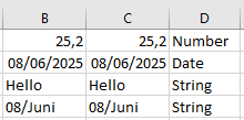
Explanation:
Assume the values shown in Figure 8.23 are in cells B1 to B4. The date in cell B4 was previously formatted.If the function IsNumeric() determines the cell content is a number, it is converted to a Double variable using CDbl().
If IsDate() finds the content to be a date, it is converted to a Date variable using CDate().
Otherwise, the cell content is assigned to a string variable.
The application can then continue working with variables of the correct data type, and—for example—output them again into a worksheet.
Retry and Cancel Buttons in Excel VBA
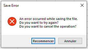
An example featuring the Retry and Cancel buttons, together with a critical warning icon, is shown in Figure.
The corresponding code is:
Sub MsgBoxRetryCancel()
    If MsgBox("An error occurred while saving the file." & vbCrLf & _
              "Do you want to try again?" & vbCrLf & _
              "Do you want to cancel the operation?", _
              vbRetryCancel Or vbCritical, _
              "Save Error") = vbRetry Then
        MsgBox "You chose to try again"
    Else
        MsgBox "You chose to cancel the operation"
    End If
End Sub
Explanation:
The Retry and Cancel buttons are combined with an icon that visually signals a critical warning.System Modal In Excel VBA
An example code of a system-modal message box is:
Sub MsgBoxSystemModal()
    MsgBox "You absolutely must read this", _
           vbOKOnly Or vbSystemModal, "Always on Top"
End Sub

Explanation:
The OK button and the vbSystemModal property are combined using the Or operator. This makes the dialog box stay always on top, even if the user switches to another application.How to use the FIXED function in Excel
This function converts numbers to formatted text with fixed decimal places and optional comma separators.
Syntax:
FIXED(number, [decimals], [no_commas])Arguments:
- number (required): The numeric value to convert
- decimals (optional):
- Positive: Rounds to specified decimal places
- Negative: Rounds left of decimal point
- Default: 2 decimal places
- no_commas (optional):
- TRUE: Omits thousands separators
- FALSE/omitted: Includes commas
Key Features:
- Conversion Rules:
- Maximum 15 significant digits
- Supports up to 127 decimal places
- Uses standard rounding (≥0.5 rounds up)
- Comparison to Formatting:
Feature FIXED() Cell Formatting Data Type Text Number Calculations Auto-converts Direct Display Fixed width Dynamic Examples:
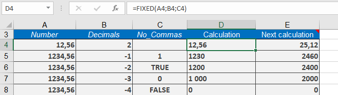
Assume that you want to ensure that a column with number values that is used for a mail merge in Word is not changed. Use the FIXED() function to convert the values into text in a new column. This column can then be used for the mail merge in Word. Here are some more examples:
=FIXED(12.56) returns 12.56.
=FIXED(1234.56,-1,1) returns 1230.
=FIXED(12.56,0) returns 13.
=FIXED(1234.56,-2,TRUE) returns 1200.
=FIXED(12.46,0) returns 12.
=FIXED(1234.56,-3,0) returns 1,000.
=FIXED(PI(),3) returns 3.142.
=FIXED(1234.56,-4,FALSE) returns 0.
Important Notes:
- For calculations, Excel automatically converts results back to numbers
- Alternative functions:
- TEXT() for custom formats
- DOLLAR() for currency formatting
- Combine with TRIM() to remove extra spaces
How to use the FIND and FINDB function in Excel
These functions locate the starting position of a substring within a text string. FIND() works with single-byte characters, while FINDB() handles double-byte characters (e.g., Asian languages). Both are case-sensitive.
Syntax:
FIND(find_text, within_text, [start_num])
FINDB(find_text, within_text, [start_byte])Arguments:
- find_text (required): The substring to search for
- within_text (required): The text to search within
- start_num/start_byte (optional):
- Character/byte position to begin search (default=1)
- First position = 1 (not 0)
Key Features:
- Case Sensitivity:
- =FIND(« E », »excel ») → #VALUE!
- =FIND(« e », »excel ») → 1
- Error Conditions:
- Returns #VALUE! if:
- Substring not found
- start_num ≤ 0
- start_num > text length
- Using wildcards (*, ?)
- Returns #VALUE! if:
- Special Cases:
- Empty find_text (« ») returns start_num
- Works with hidden characters
Comparison with SEARCH():
Feature FIND() SEARCH() Case-Sensitive Yes No Wildcards No Yes Error Handling Strict Flexible EXAMPLE
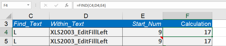
Assume that you have a string that is separated into two parts by an underscore. If you want to locate the uppercase S in the second part of the string and find its position in the string, you will first need to determine the position of the underscore to ensure that the first part is not searched.
Then you can perform the search in the remainder of the string. If cell C19 contains the string XLS2003_FormatCellSecure, the formula
=FIND(« S »,C19,FIND(« _ »,C19)+1)
returns 17, because the S in the second part of the string is located in the nineteenth position
Notes:
- For case-insensitive searches, use SEARCH()
- Combine with LEFT/RIGHT/MID for text extraction
- FINDB() essential for double-byte character systems
How to use the EXACT function in Excel
This function performs a case-sensitive comparison of two text strings, returning TRUE if they are identical and FALSE otherwise.
Syntax:
EXACT(text1, text2)Arguments:
- text1 (required): First text string for comparison
- text2 (required): Second text string for comparison
Key Features:
- Case Sensitivity:
- =EXACT(« Word », « word ») → FALSE
- =EXACT(« Word », « Word ») → TRUE
- Format Ignorance:
- Only compares raw text content
- Ignores font styles, colors, or cell formatting
- Array Compatibility:
- Can compare a value against a range using array formulas
Practical Applications:
- Data Validation:
=EXACT(A2, PROPER(A2)) // Checks for proper capitalization
- Password Verification:
=EXACT(B1, B2) // Compares two password entries
- Array Search (Ctrl+Shift+Enter):
{=OR(EXACT(D22,B23:B48))} // Checks if D22 exists in range
Comparison with Equal Sign (=):
Feature EXACT() = Operator Case-Sensitive Yes No Format-Aware No No Array-Friendly Yes Limited Examples:
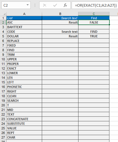
Assume that after you have entered a list of data, you want to examine the array to check whether it contains a specific character string. The list is entered in the cell range B23:B48, and cell D22 contains the search string. Enter the following formula in a cell:
=OR(EXACT(C1;A2:A27))
and press Ctrl+Shift+Enter. The formula looks like this (see Figure 8-3):
{=OR(EXACT(C1;A2:A27))}
If you use the function as an array expression, you need the OR() function to return a single value from the list.
Here are a few further examples:
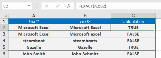
=EXACT(« Microsoft Excel », »Microsoft excel ») returns FALSE.
=EXACT(« steamboat », »steamboats ») returns FALSE.
=EXACT(« gazelle », »gazelle ») returns TRUE.
=EXACT(« John Smith », »Jeff Smith ») returns FALSE.
Limitations:
- Does not support wildcards (*, ?)
- For case-insensitive checks, use =A1=B1
- Array formulas require Ctrl+Shift+Enter in Excel 2019
How to use the DOLLAR function in Excel
This function converts a numeric value to text formatted as currency, using the local currency symbol and formatting conventions.
Syntax:
DOLLAR(number, [decimals])Arguments:
- number (required):
The numeric value to convert (can be a number, cell reference, or formula) - decimals (optional):
Number of decimal places to display:- Positive: Rounds to specified decimal places
- Negative: Rounds left of decimal point
- Omitted: Defaults to 2 decimal places
Key Features:
- Conversion Behavior:
- Converts numbers to text strings with currency formatting
- Uses local currency symbol based on system settings
- Default format: $#,##0.00;($#,##0.00)
- Comparison to Cell Formatting:
Feature DOLLAR() Format Cells Data Type Text Number Display Overflow Truncates Shows ### Calculations Auto-converts Directly usable - Rounding Rules:
- Uses standard rounding (≥0.5 rounds up)
- Negative decimals round to 10s, 100s, etc.
Examples:
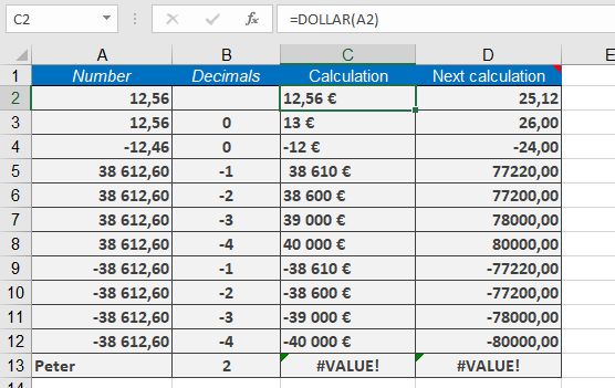
Assume that you want to ensure that a price column used for a mail merge in Microsoft Word is not changed. For this reason, you use the DOLLAR() function to convert the values in the price column into the corresponding currency text in a calculated column. The calculated column is used for the mail merge process in Word. Here are some other examples:
=DOLLAR(12.56) returns $12.56.
=DOLLAR(38612.60,-1) returns $38,610.
=DOLLAR(12.56,0) returns $13.
=DOLLAR(38612.60,-2) returns $38,600.
=DOLLAR(12.46,0) returns $12.
=DOLLAR(38612.60,-3) returns $39,000.
=DOLLAR(PI(),3) returns $3.142.
=DOLLAR(38612.60,-4) returns $40,000.
As shown below;
- number (required):