Votre panier est actuellement vide !
Catégorie : Excel function
How to Use the OR Function in Excel
The OR function is a logical function that returns TRUE if any of the specified conditions are TRUE, and returns FALSE only if all conditions are false. Unlike the AND function, which requires all conditions to be true, the OR function only needs one true condition to return TRUE.
The syntax for the OR function is as follows:
=OR(logical1; [logical2]; …)
- logical1 (Required): The first condition or logical value to evaluate.
- logical2 (Optional): The second condition or logical value to evaluate.
USING THE OR FUNCTION
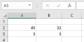
Let’s determine whether:
- Cell A2 is greater than 30,
- Cell B2 is less than 50,
- Cell B3 is equal to 45,
by using the OR function to return either TRUE or FALSE based on the evaluation.
To apply the function:
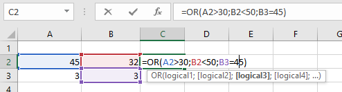
- Select an empty cell and enter the function with the specified arguments:
=OR(A2>30; B2<50; B3=45)
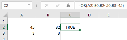
- Press Enter, and the result will be displayed (e.g., FALSE if none of the conditions are met).
NOTES WHEN USING THE OR FUNCTION
- If any logical test cannot be interpreted as a numeric or logical value, the function returns a #VALUE! error.
- The function ignores text values or empty cells in the arguments.
- It can evaluate up to 255 conditions in a single function.
- The OR function can also be combined with the AND function, depending on the required logic.
How to Use the IFERROR Function in Excel
The IFERROR function is used to return a custom result when a formula produces an error. It provides a simple way to handle errors without complex nested IF statements.
The IFERROR function uses the following syntax:
=IFERROR(value; value_if_error)
Arguments:
- Value (Required): The formula or expression to be checked for errors
- Value_if_error (Required): The result to return if an error is detected
USING THE IFERROR FUNCTION
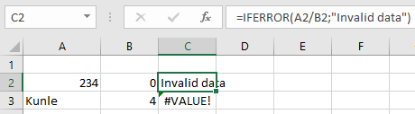
Using the table below, we’ll apply the IFERROR function to replace errors with the message « invalid data »:
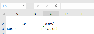
To correct the error in cell C2:
- Select an empty cell
- Enter the formula:
=IFERROR(A2/B2; « invalid data »)
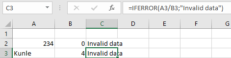
To correct the error in cell C3:
- Select an empty cell
- Enter the formula:
=IFERROR(A3/B3; « invalid data »)
IMPORTANT NOTES ABOUT THE IFERROR FUNCTION
- If either value or value_if_error refers to an empty cell, IFERROR treats it as an empty string (« »)
- When applied to an array formula, IFERROR returns an array of results for each cell in the specified range
- Common errors handled by IFERROR include:
- #N/A
- #VALUE!
- #REF!
- #DIV/0!
- #NUM!
- #NAME?
- #NULL!
The IFERROR function simplifies error handling in formulas while maintaining spreadsheet clarity and efficiency.
How to Use the IFS Function in Excel
The IFS function serves as an alternative to nested IF functions. This function evaluates one or more conditions and returns the value corresponding to the first TRUE condition found.
The IFS function operates using the following syntax:
=IFS(Logical_test1; Value1; [Logical_test2, Value2]; …; [Logical_test127; Value127])
Arguments:
- Logical_test1 (Required): The first condition Excel evaluates as TRUE or FALSE
- Value1 (Required): The result returned if Logical_test1 is TRUE
- Additional logical tests and values (Optional): You can include up to 127 condition/value pairs
USING THE IFS FUNCTION
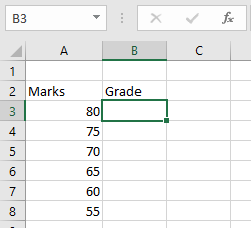
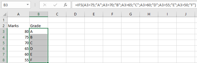
Let’s apply the IFS function to assign letter grades based on student marks from the table below:
To assign grades:
- Select an empty cell
- Enter the formula:
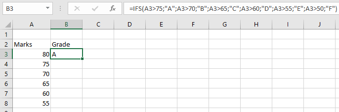
=IFS(A3>75; »A »; A3>70; »B »; A3>65; »C »; A3>60; »D »; A3>55; »E »; A3>50; »F »)
- Press Enter to see the grade for the first student
To apply this to other students:
- Use the fill handle to drag the formula down to adjacent cells
IMPORTANT NOTES ABOUT THE IFS FUNCTION
- #N/A Error: Occurs when none of the specified conditions are met
- #VALUE! Error: Appears when a logical test returns a value that isn’t TRUE or FALSE
- Evaluation Order: The function checks conditions sequentially and stops at the first TRUE result
- Default Case: Unlike IF, IFS doesn’t have a built-in « else » clause – all possible outcomes must be explicitly defined
How to Use the NESTED IF Function in Excel
The Nested IF function refers to one IF function placed inside another IF function, enabling you to evaluate multiple conditions and expand the range of possible results. While you could achieve similar outcomes using separate IF functions individually, nesting them provides a more streamlined approach. Now, let’s apply the Nested IF function to the table below to examine whether prices exceed or fall below 500.

USING THE NESTED IF FUNCTION
To determine if a value is greater than 500 using the Nested IF, input the following formula in an empty cell:
=IF(A2>500; « Yes »; « No »
=IF(A3>500; « Yes »; « No »
=IF(A4>500; « Yes »; « No »
=IF(A5>500; « Yes »; « No »)
=IF(A6>500; « Yes »; « No »))))
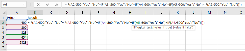
Press Enter, and the result for the first referenced cell will appear.
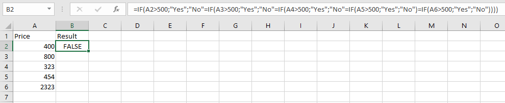
To extend this evaluation to the remaining cells, utilize the fill handle to drag the formula downward, applying it to the other cells automatically.

IMPORTANT NOTES ON NESTED IF FUNCTIONS
- Precision in Construction
- Crafting a Nested IF function demands careful thought and accuracy to ensure the logic processes each condition correctly through to the final outcome.
- Potential for Complexity
- Nested IF functions can become difficult to follow, particularly when numerous IF functions are nested within one another.
- Precision in Construction
How to Use the IF Function in Excel
The IF function is a function that tests a given condition and returns one value for a TRUE result and another value for a FALSE result. This function allows you to make a logical comparison between a value and what you expect.
The IF function uses the following syntax:
=IF(Logical_test; [Value_if_true]; [Value_if_false])
Arguments:
- Logical_test (Required Argument): This is the value or logical expression to be tested and evaluated as either TRUE or FALSE.
- Value_if_true (Optional Argument): This is the value returned if the logical test evaluates to TRUE.
- Value_if_false (Optional Argument): This is the value returned if the logical test evaluates to FALSE.
When using this function, the following logical operators can be applied:
- Equal to (=)
- Greater than (>)
- Greater than or equal to (≥)
- Less than (<)
- Less than or equal to (≤)
- Not equal (≠)
USING THE IF FUNCTION
In the table below, we want to test whether the values in the cells are greater than 500 or not. If TRUE, the result will be « Yes », and if FALSE, the result will be « No ».
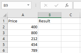
To check if cell A2 is greater than 500, enter:
=IF(A2>500; « Yes »; « No »)
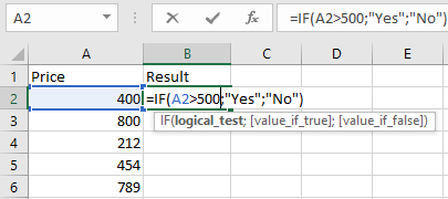
Press Enter, and the returned value will be « No ».
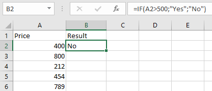
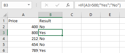
Use the same steps to evaluate cells A3 to A6:
=IF(A3>500; « Yes »; « No »)
=IF(A4>500; « Yes »; « No »)
=IF(A5>500; « Yes »; « No »)
=IF(A6>500; « Yes »; « No »)
NOTES WHEN USING THE IF FUNCTION:
- The IF function works if the logical_test returns a numeric value.
- It treats any non-zero value as TRUE and zero as FALSE.
- #VALUE! occurs when the logical_test argument cannot be evaluated as TRUE or FALSE.
- If any argument is supplied as an array, the IF function evaluates each element of the array.
- To count based on conditions, use COUNTIF and COUNTIFS.
- To sum based on conditions, use SUMIF and SUMIFS.
How to Use the REFERENCE FORMAT OF THE INDEX Function in Excel
The reference format of the INDEX function returns a cell reference at the intersection of specified row and column numbers within one or more ranges.
Syntax:
=INDEX(reference; row_num; [column_num]; [area_num])
Arguments:
- reference (Required):
One or more cell ranges. Multiple ranges must be separated by commas and enclosed in parentheses (e.g., (A1:B2;D5:E6)). - row_num (Required):
The row position within the reference.- If 0, returns a reference to all rows in the range.
- column_num (Optional):
The column position within the reference.- If 0, returns a reference to all columns in the range.
- area_num (Optional):
Specifies which range to use when multiple ranges are provided in reference.- Defaults to 1 (first range) if omitted.
USING THE REFERENCE FORMAT OF THE INDEX FUNCTION
Example: Find the Price of Mango
Given the following table (range A2:C10):
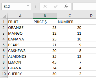
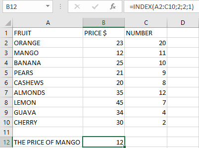
Steps to find Mango’s price (row 2, column 3, area 1):
- Select an empty cell.
- Enter the formula:
=INDEX((A2:C10); 2; 3; 1)
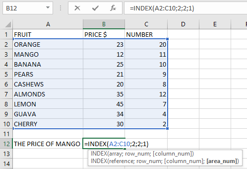
- Press Enter → Returns 12 (Mango’s price).
NOTES & ERROR HANDLING
- Return Behavior:
- Returns the value at the row/column intersection when both row_num and column_num are specified.
- Returns an array of values if either row_num or column_num is 0.
- Common Errors:
- #VALUE!: Occurs if row_num, column_num, or area_num is non-numeric.
- #REF!: Occurs when:
- row_num exceeds the range’s row count.
- column_num exceeds the range’s column count.
- area_num exceeds the number of provided ranges.
- Multi-Range Example:
=INDEX((A1:B2;D5:E6); 1; 2; 2)
Returns the value from row 1, column 2 of the second range (D5:E6).
- reference (Required):
How to use the INDEX function in Excel
The INDEX function returns a value or reference from within a table or range based on specified row and column positions. This function is commonly used with MATCH and can serve as an alternative to VLOOKUP. The INDEX function has two formats:
- Array Format
- Reference Format
THE ARRAY FORMAT OF THE INDEX FUNCTION
The array format returns the value of a specific cell or range of cells within an array.
Syntax:
=INDEX(array; row_num; [col_num])
Arguments:
- array (Required):
The range of cells to search within. - row_num (Required):
The row position in the array to return.- If set to 0 or omitted, returns all rows in the array.
- col_num (Optional):
The column position in the array to return.- If set to 0 or omitted, returns all columns in the array.
USING THE ARRAY FORMAT OF THE INDEX FUNCTION
Example: Find Goals Scored by LOVETH
Given the following table (range A2:C5):
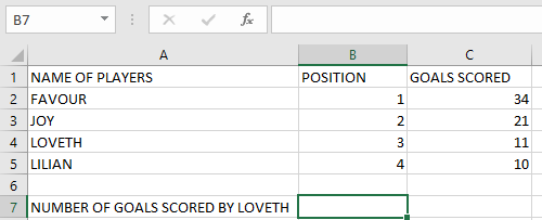
Steps to find Loveth’s goals (row 3, column 3):
- Select an empty cell.
- Enter the formula:
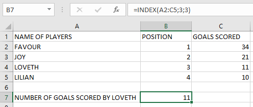
=INDEX(A2:C5; 3; 3)

- Press Enter → Returns 11 (Loveth’s goals).
How to use the ROW function in Excel
The ROW function returns the row number of a specified cell reference in a worksheet. This function helps identify the numerical position of rows in Excel’s grid system.
Syntax:
=ROW([reference])
Argument:
- reference (Optional):
The cell or range for which you want to determine the row number.- If omitted, returns the row number of the cell containing the formula.
USING THE ROW FUNCTION
Example: Finding Row Numbers
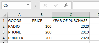
To find the row number of cell A3:
- Select a blank cell
- Enter the formula:
=ROW(A3)
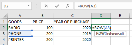
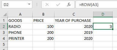
- Press Enter → Returns 3
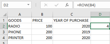
To find the row number of cell B4:
- Select a blank cell
- Enter the formula:
=ROW(B4)
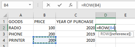
- Press Enter → Returns 4
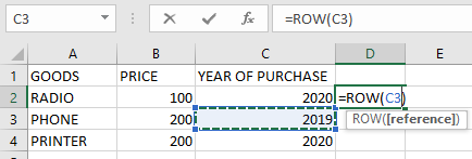
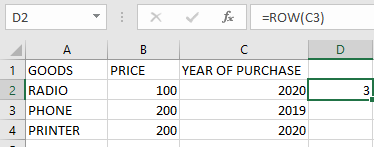
To find the row number of cell C3:
- Select a blank cell
- Enter the formula:
=ROW(C3)
- Press Enter → Returns 3
Using ROW without reference:
=ROW()
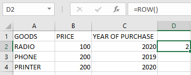
Returns the row number of the cell containing this formula.
IMPORTANT NOTES:
- Single Reference Only:
- Processes only one cell reference at a time
- Reference Types Accepted:
- Works with single cells or range references
- Returns the top row number for ranges
- Optional Argument:
- When omitted, automatically references the formula cell
- Array Handling:
- Returns an array of row numbers when reference is a range
- Example: =ROW(A1:A5) returns {1;2;3;4;5}
- Key Differences from ROWS Function:
- ROW returns position numbers
- ROWS counts total rows in range
- reference (Optional):
How to use the COLUMN function in Excel
The COLUMN function returns the column number of a specified cell reference within a worksheet. This function provides the numerical position of a column in Excel’s grid system.
Syntax:
=COLUMN([reference])
Argument:
- reference (Optional):
The cell or range for which you want to determine the column number.- If omitted, returns the column number of the cell containing the formula.
USING THE COLUMN FUNCTION
Example: Finding Column Numbers
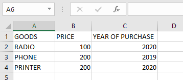
To find the column number of cell A4:
- Select a blank cell
- Enter the formula:
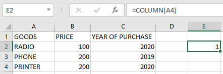
=COLUMN(A4)
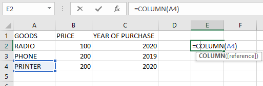
- Press Enter and the column number will be displayed
To find the column number of cell B3:
- Select a blank cell
- Enter the formula:
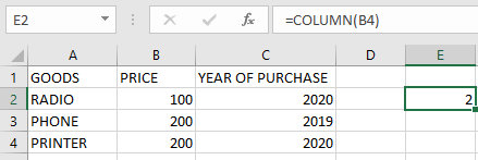
=COLUMN(B4)
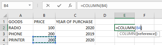
- Press Enter → Returns 2 (B is the second column)
To find the column number of cell C1:
- Select a blank cell
- Enter the formula:
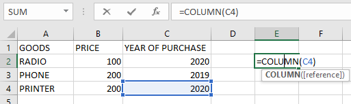
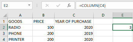
=COLUMN(C4)
- Press Enter → Returns 3 (C is the third column)
Using COLUMN without reference:
=COLUMN()
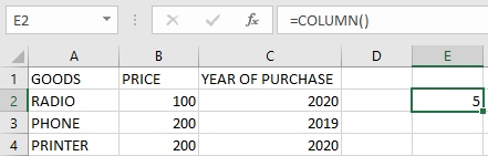
Returns the column number of the cell containing this formula.
IMPORTANT NOTES:
- Single Reference Only:
- Cannot process multiple cell references simultaneously
- Reference Types Accepted:
- Works with single cells or range references
- Returns the leftmost column number for ranges
- Optional Argument:
- When omitted, automatically references the formula cell
- Practical Applications:
- Useful in combination with other functions like INDEX, OFFSET
- Helps create dynamic column references in formulas
- reference (Optional):
How to use the FORMULATEXT function in Excel
The FORMULATEXT function displays the formula contained in a specified cell as a text string. This function was introduced in Microsoft Excel 2013.
Syntax:
=FORMULATEXT(reference)
Argument:
- reference (Required):
The cell reference containing the formula you want to display as text.
USING THE FORMULATEXT FUNCTION
Example: Display a Cell’s Formula
Given a cell (B7) containing a formula to calculate Joy’s mathematics score:
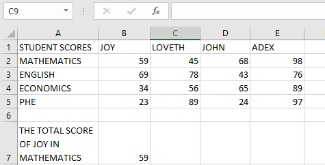
Steps to Display the Formula:
- Select an empty cell type in the function =FORMULATEXT
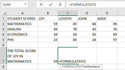
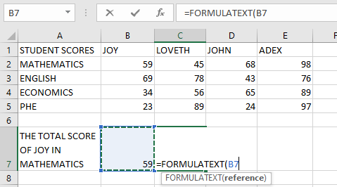
- Enter the function:
=FORMULATEXT(B7)
- Press Enter
Result:
The actual formula from cell B7 will be displayed as text in the selected cell.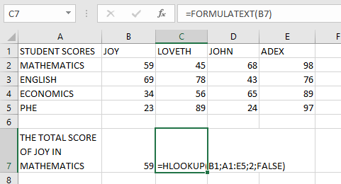
ERRORS & IMPORTANT NOTES
Common Errors:
- #VALUE! Error:
Occurs when invalid data types are used as inputs. - #N/A Error:
Occurs when:- The referenced cell doesn’t contain a formula
- Referencing a closed workbook
- The formula exceeds 8192 characters
- The worksheet is protected
Key Points:
- Only displays formulas – won’t show values or text
- Particularly useful for:
- Documenting complex spreadsheets
- Troubleshooting formulas
- Auditing workbook calculations
- reference (Required):