Votre panier est actuellement vide !
Étiquette : practical-excel
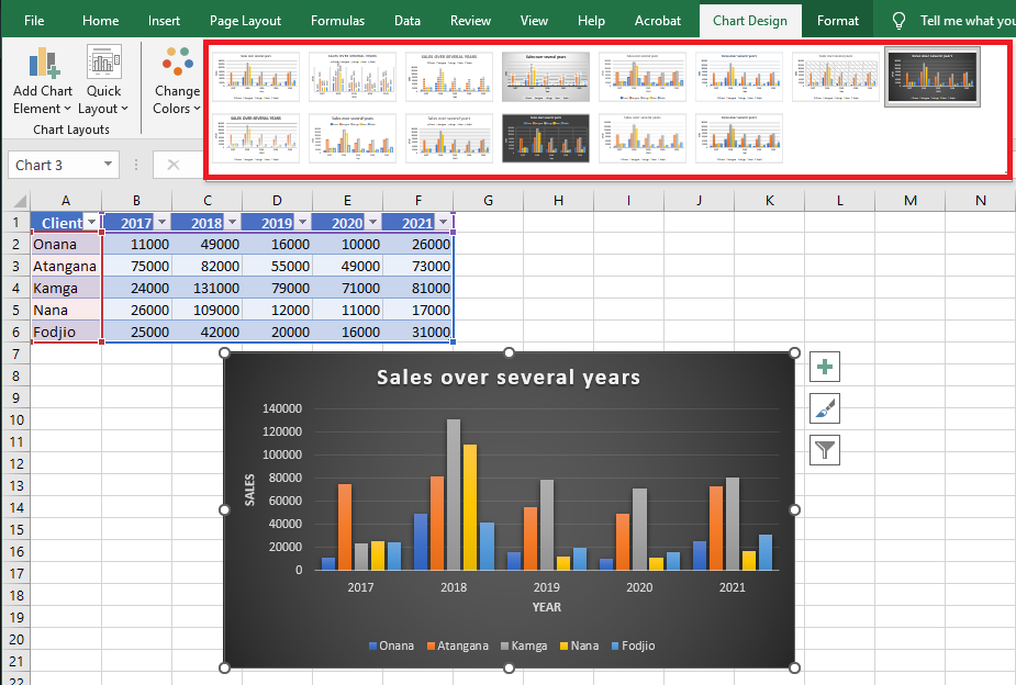
Apply Chart Layouts and Styles in Excel
A simple way to change the appearance of a chart is to apply one of the built-in layouts or styles available in Excel.
Apply a Chart Layout
Built-in chart layouts quickly adjust the overall layout of a chart by combining titles, labels, and orientations.
-
Select the chart you want to format.
-
Click the Design tab.
-
Click the Quick Layout button.
-
Choose a layout from the list.
 The selected layout is applied to the chart.
Apply a Chart Style
Built-in chart styles allow you to adjust the format of multiple chart elements at once.
Styles quickly change colors, shading, and other formatting properties.-
Select the chart.
-
Click the Design tab.
-
Click the More Chart Styles button.
If the style you want is already shown in the gallery, you don’t need to expand the menu—just click to apply it. - Select a new style.
The new style is applied to the chart.
Change the Chart Colors
You can keep the overall style while updating only the colors to better suit your needs.
-
Select the chart.
-
Click the Design tab.
-
Click the Change Colors button.
- Select a new color palette.

The new color scheme is applied to the chart.
NOTE:
You can also access chart styles and colors using the Chart Styles icon (paintbrush) that appears to the right of the chart when selected.
The dropdown list shows the same choices as in the Chart Tools / Design / Chart Styles group.-
Add and Modify Chart Elements in Excel
Chart elements provide more context and description to your charts, making your data more meaningful and visually appealing. In this section, you’ll learn about chart elements.
Follow the steps below to insert chart elements into your chart. When you click on the chart, three buttons appear in the upper-right corner:
- Chart Elements
- Chart Styles and Colors
- Chart Filters
Clicking on the Chart Elements icon displays a list of available elements:
- Axes
- Axis Titles
- Chart Title
- Data Labels
- Data Table
- Error Bars
- Gridlines
- Legend
- Trendline
You can add, remove, or modify any of these chart elements.
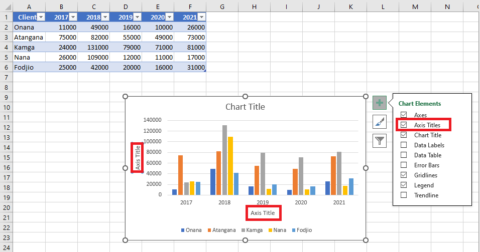
Hover over each chart element in the list to preview how it will appear. For example, selecting Axis Titles highlights both the horizontal and vertical axis titles.
A small triangle appears next to Axis Titles in the list. Click the triangle to see available options.
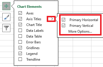
Check or uncheck the elements you want to display on your chart.
Axes
Charts usually have two axes used to measure and categorize data:
- A vertical axis (also called value axis or Y-axis)
- A horizontal axis (also called category axis or X-axis)

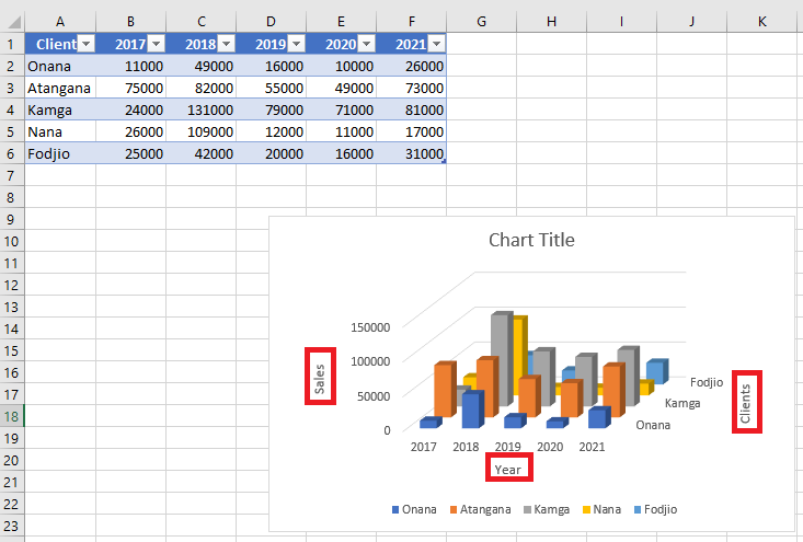
3D column charts include a third axis, the depth axis (also called series axis or Z-axis), and data can be plotted along this depth.

Radar charts don’t have horizontal/category axes. Pie and doughnut charts do not have axes at all.
Not all chart types display axes the same way:
- XY scatter charts and bubble charts display numeric values on both the X and Y axes.
- Column, line, and area charts display numeric values on the Y-axis and text groupings (categories) on the X-axis.
- The depth axis is another form of category axis.
Axis Titles
Axis titles help users understand what the axes in a chart represent.
- You can add axis titles to horizontal, vertical, or depth axes.
- You cannot add axis titles to charts without axes (e.g., pie or doughnut charts).
To add axis titles:
- Click on the chart.
- Click the Chart Elements (+) icon.
- Select Axis Titles from the list.

- Axis titles appear on the chart for each axis. Click on an axis title to edit it and enter meaningful labels.
You can also link axis titles to cells in the worksheet. When the cell’s text changes, the axis title updates automatically:
- Click on any axis title in the chart.
- In the formula bar, type an equal sign
=and then select the worksheet cell containing the desired text. - Press Enter.
 The axis title now displays the content of the linked cell.
Chart Title
When you create a chart, a Chart Title box appears at the top.
To add or change a chart title:
- Click on the chart.
- Click the Chart Elements icon.
- In the list, select Chart Title.

- A chart title box appears. Click in the box and type your desired title.

You can also link the chart title to a worksheet cell:
- Click on the chart title.
- In the formula bar, type
=and select the cell with the desired text. - Press Enter. The chart title will now reflect the cell’s content and update automatically when the cell’s value changes.
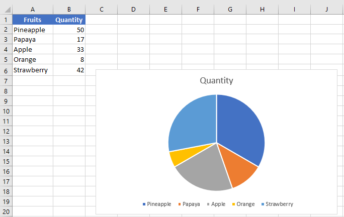
Data Labels
Data labels enhance a chart by showing details of each data point.
Example: In a pie chart, you may notice that pineapples and papayas have the largest slices, but it’s unclear what the exact values are.
To add data labels:
- Click on the chart.
- Click the Chart Elements icon.
- Select Data Labels from the list. Labels now appear on each slice of the pie.
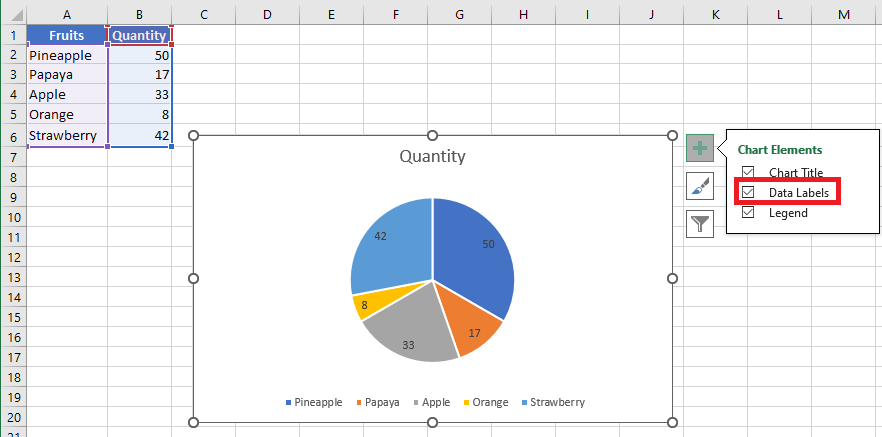
Now you can clearly read: 50 pineapples, 42 papayas, and 33 apples.
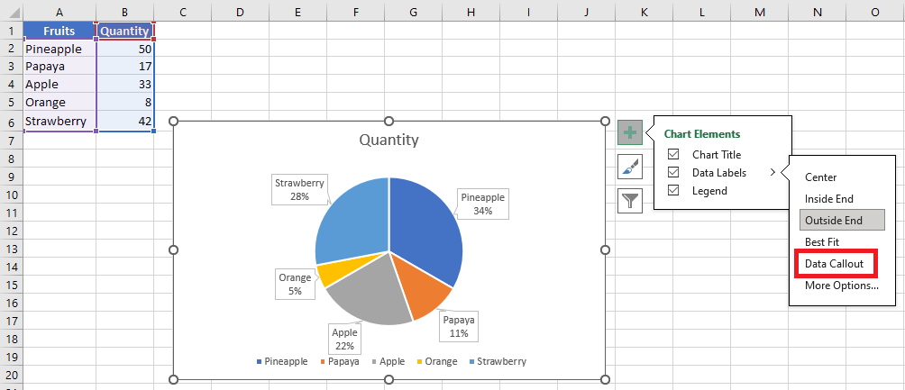
You can change the label position:
- Click the triangle next to Data Labels to see placement options.
- Hover over each option to preview the layout (e.g., outside end, center, etc.).
Data Table
Data tables can be added to line, area, column, and bar charts.
To insert a data table:
- Click on the chart.
- Click the Chart Elements icon.
- Select Data Table from the list. A table appears below the chart, replacing the horizontal axis with a header row.
In bar charts, the data table is aligned with the chart but doesn’t replace an axis.
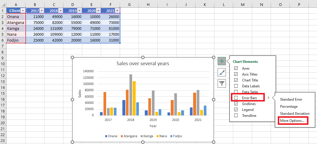
Error Bars
Error bars graphically represent potential error margins in each data point.
Example: Show ±5% margins in scientific experiment results.
You can add error bars to series in 2D area, bar, column, line, scatter, and bubble charts.
To insert error bars:
- Click on the chart.
- Click the Chart Elements icon.
- Select Error Bars. Click the triangle to view more options.
- Click More Options… to open the error bar settings dialog.
- Select the data series and click OK.
 Error bars will now appear for the selected series.
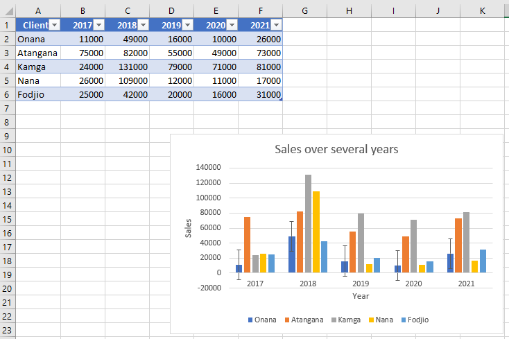
If you modify values in the worksheet, the error bars adjust automatically.
For scatter and bubble charts, you can show error bars for X values, Y values, or both.
Gridlines
Gridlines help interpret chart data by extending from axes across the chart plot area. You can display horizontal, vertical, and depth gridlines (in 3D charts).
To insert gridlines:
- Click on the 3D column chart.
- Click the Chart Elements icon.
- Select Gridlines from the list. Click the triangle to see all gridline types.
- Select Primary Major Horizontal, Primary Major Vertical, and Primary Major Depth.
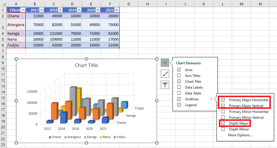
Gridlines appear on the chart accordingly.
Note: Gridlines cannot be added to chart types without axes, such as pie or doughnut charts.
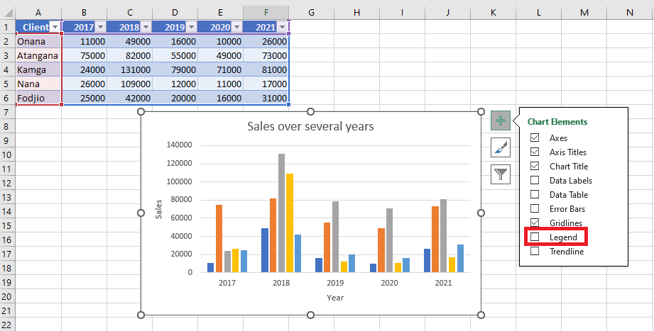
Legend
When you create a chart, the legend appears by default.
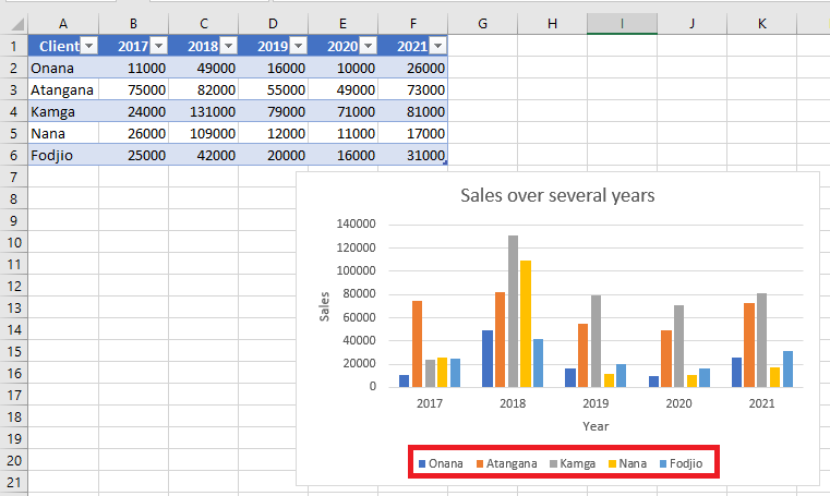
To hide it, simply uncheck Legend in the Chart Elements list.
Trendline
Trendlines are used to visualize trends and perform predictive analysis (also called regression analysis).
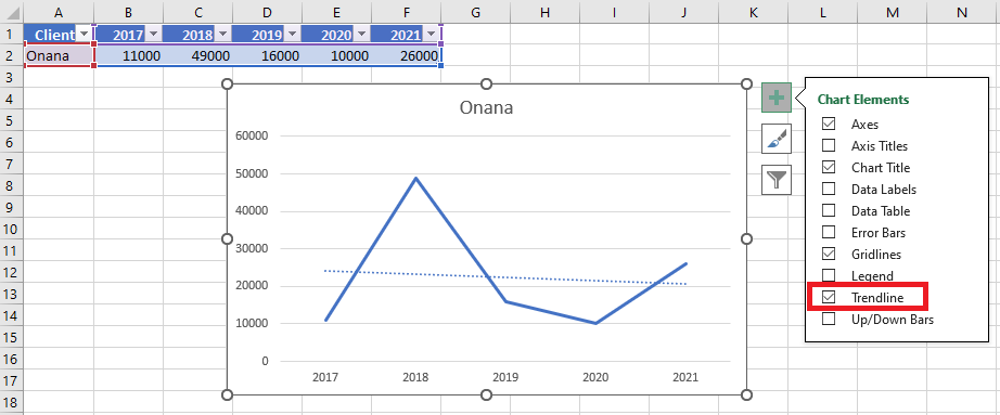
You can extend a trendline beyond existing data points to forecast future values based on historical trends.
Resizing Charts in Excel
After creating your chart, you may want to adjust its size to fit a specific location on your worksheet.
There are three methods to resize your chart:
Start by activating your chart by clicking on it, then proceed to resize it using one of the three methods described below:Method 1
Click one of the handles around the selected chart and drag inward or outward until you reach the desired size.Method 2
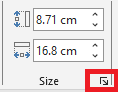
Use specific height and width measurements.
If you want to define custom height and width values, click the Format tab on the ribbon, then manually enter your measurements in the Height and Width fields in the Size group.
Method 3
Use the Format Chart Area dialog box:
First, display this dialog box using one of the following methods:- Click the dialog box launcher in the Size group.
- Right-click the chart area and choose Format Chart Area.
- Double-click on the chart area.
In the Format Chart Area dialog box, click the Size & Properties tab.
In the Size section, enter your desired Height and Width values.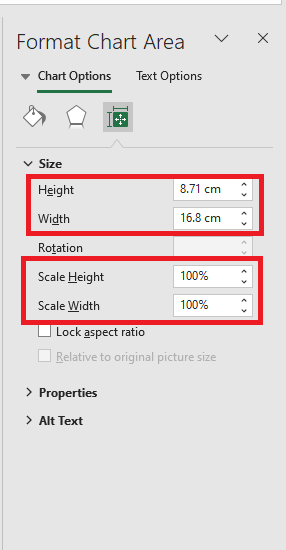
You can also use the Scale Height and Scale Width options to resize your chart by a specific percentage.
Maintain Aspect Ratio
Check this box to maintain proportional resizing between width and height.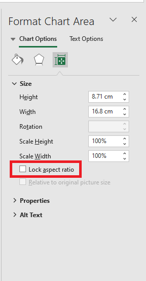
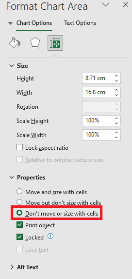
Keep Chart Size and Position Independent from Cells
When you resize cells underneath your chart or when you hide or resize rows or columns, it may affect the chart’s size.To keep the chart size independent of any changes made to those cells (rows or columns), click on Properties in the Format Chart Area dialog box and select the option Don’t move or size with cells.
Analyze Data Using Quick Analysis in Excel
The Quick Analysis tools in Excel are features provided to help you analyze data instantly, rather than using the traditional method of manually inserting a chart or table. A yellow Quick Analysis box appears at the bottom right corner of the selection—or you can press CTRL + Q to open the Quick Analysis tools.
Quickly calculate totals, insert tables, apply conditional formatting, and more.
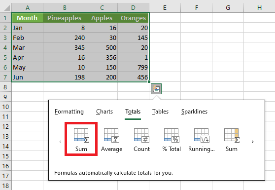
Totals
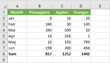
Instead of manually adding a total row at the end of an Excel table, use the Quick Analysis tool to calculate totals instantly.
- Select a range of cells and click the Quick Analysis button.
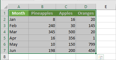
- For example, click Totals, then click Sum to add up the numbers in each column.
Result:
Select the range A1:D7 and add a column with a running total.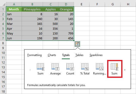
NOTE:
Total rows are highlighted in blue, and total columns appear in yellow-orange.
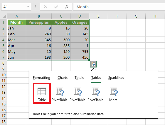
Tables
Use tables in Excel to sort, filter, and summarize data. A PivotTable in Excel lets you extract meaning from a large, detailed dataset.
- Select a range of cells and click the Quick Analysis button.
- To quickly insert a table, click Tables, then click Table.
Result:
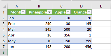
A structured Excel table is created with filter controls and automatic formatting.Formatting
Data bars, color scales, and icon sets in Excel make it easy to visualize the values in a cell range.
- Select a range of cells and click the Quick Analysis button.
- To quickly add data bars, click Data Bars.
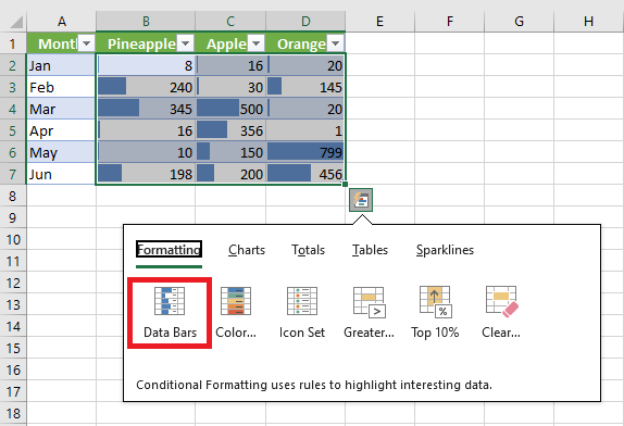
A longer bar represents a higher value.
- To quickly add a color scale, click Color Scale.
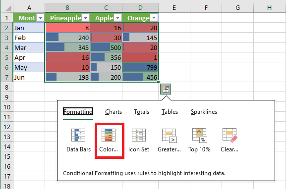
The shade of the color reflects the value in the cell.- To quickly add an icon set, click Icon Set.
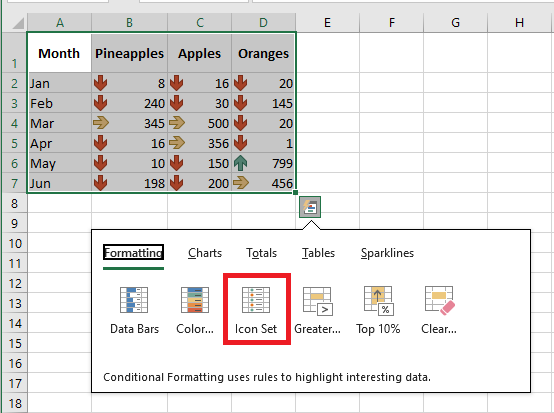
Each icon represents a range of values.
- To quickly highlight cells greater than a certain value, click Greater Than.
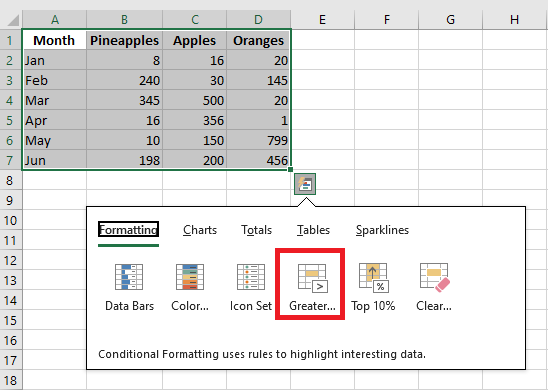
- Enter the value 200 and select a formatting style.
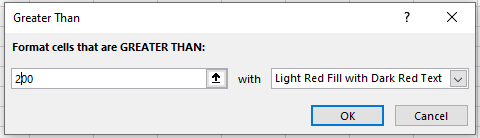
- Click OK.
Result:
Excel highlights cells with values greater than 200.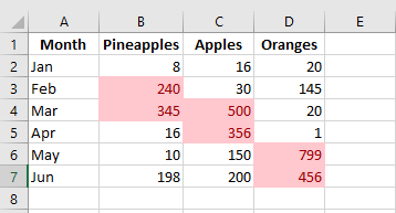
Charts
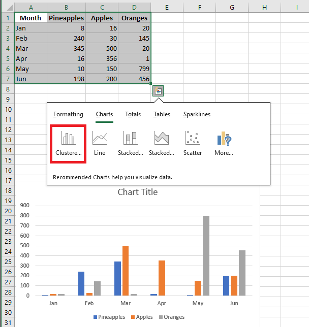
You can use the Quick Analysis tool to create a chart instantly. The Recommended Charts feature analyzes your data and suggests useful chart types.
- Select a range of cells and click the Quick Analysis button.
- For example, click Charts, then click Clustered Column to create a grouped column chart.
Sparklines
Sparklines in Excel are miniature charts that fit inside a single cell. They are ideal for showing trends.
- Select the range A1:F4 and click the Quick Analysis button.
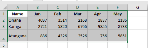
- For example, click Sparklines, then click Line to insert sparklines.
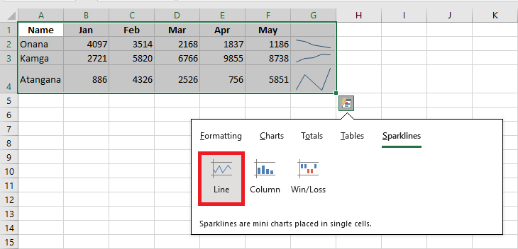
Custom Result:
Each selected row gets a compact line graph showing the evolution of values across the row.Switching Rows and Columns in Source Data in Excel
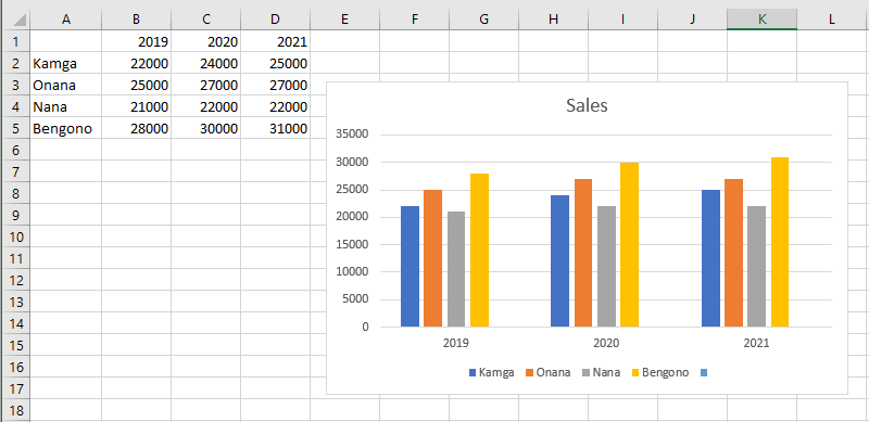
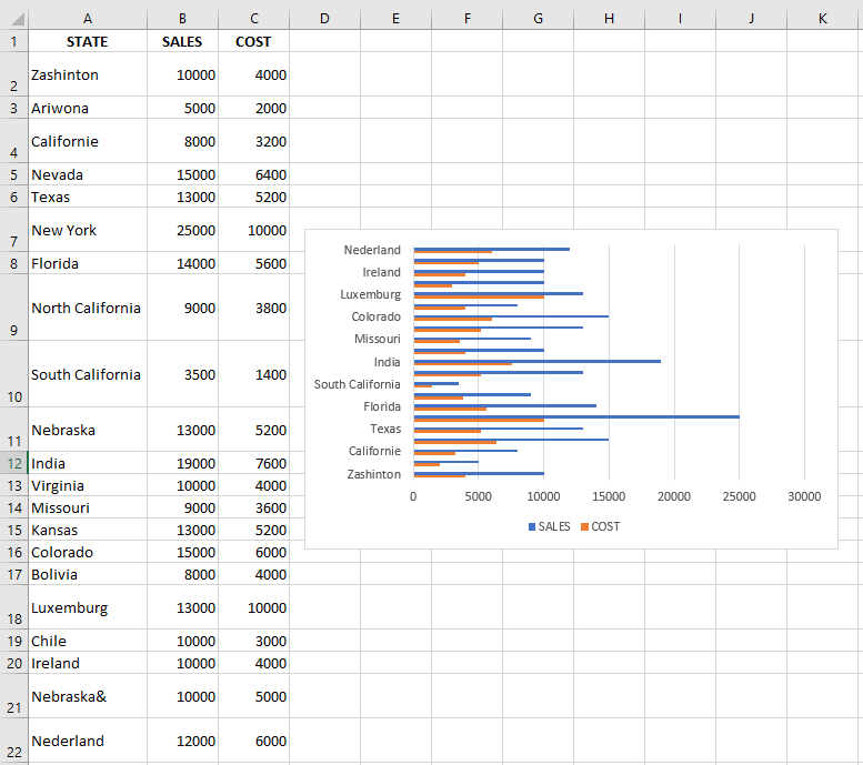
Switching rows and columns in your data can be useful if the layout of the worksheet data is not ideal. It can also give you an alternative chart layout, which may be more suitable depending on how you intend to use your chart. This feature allows you to swap your legend entries (series) with your horizontal axis labels (categories).
Note: This only works with a single data series, so I removed the Costs series for this example.
To switch rows and columns in your chart:
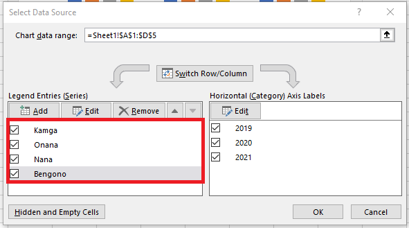
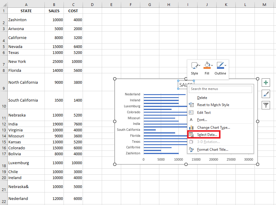
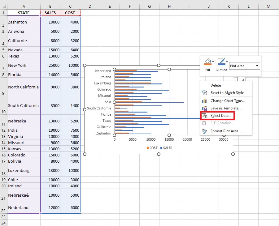
- Right-click the chart and select Select Data.
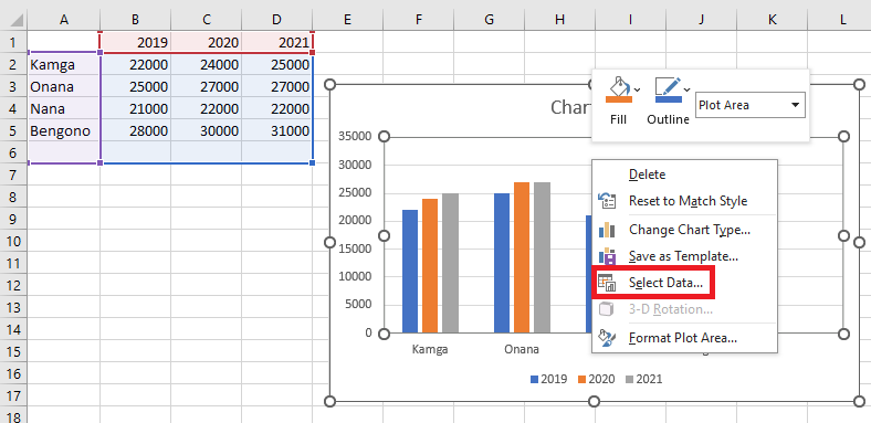 Here is what the Select Data Source window looks like:
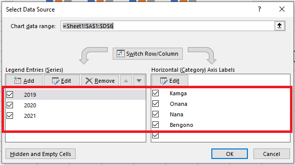
- Then click the Switch Row/Column button, and click OK to update the chart.
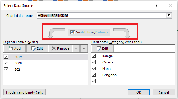
Notice how the states are now my legend key, and the sales are on my Y-axis, with the legend entries / horizontal axis labels switched.
Other Methods
A quicker alternative method:
- Click the Chart Design tab.
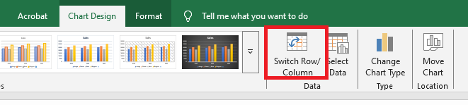
- Click the Switch Row/Column button.
- The rows are now converted to columns.
Adding Additional Data Series in Excel
After creating a chart, you may need to add a data series to it. A data series is a row or column of numbers entered in a worksheet and plotted in your chart—for example, a list of the company’s quarterly profits.
Office charts are always linked to an Excel worksheet, even if you created your chart in another program such as Word. If your chart is located on the same worksheet as the data used to create it (also called the source data), you can quickly drag the pointer around the new data in the worksheet to include it in the chart. If your chart is on a separate sheet, you’ll need to use the Select Data Source dialog box to add a data series.
Quickly Adding Data Series
To quickly add a data series to a chart on the same worksheet:
In the worksheet that contains your chart’s data, in the cells directly next to or below your existing chart data, enter the new data series you want to add.
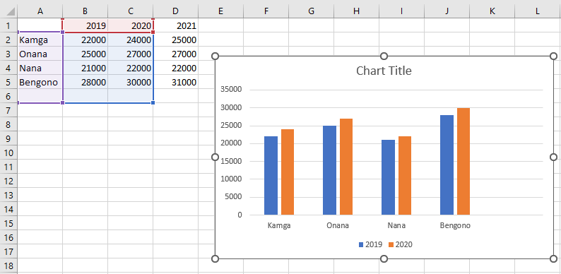
In this example, we have a chart that shows 2019 and 2020 quarterly sales data, and we’ve just added a new 2021 data series to the worksheet. Note that the chart does not yet display the 2021 series.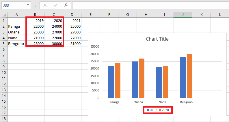
Click anywhere on the chart.
The currently displayed source data is selected in the worksheet, with resizing handles visible.
You’ll notice that the 2021 data series is not selected.
In the worksheet, drag the resizing handles to include the new data.
The chart updates automatically and displays the new data series you added.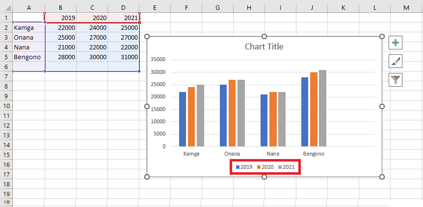
Other Methods to Add Data Series
To add another data series to your chart, right-click the chart and select Select Data.
The following dialog box appears.
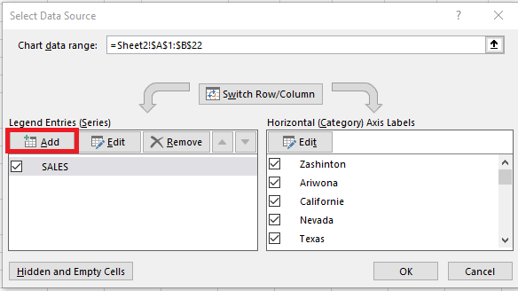
Click the Add button. The next window will open:
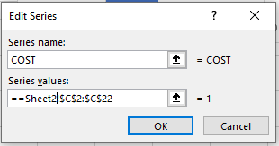
This allows you to select a new series name and reference the cells that contain the new series data. Click OK to update the chart.

Deleting Data from a Chart
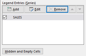
To remove a data series, select it and then click the Remove button.
For example, I will remove the data series I just added: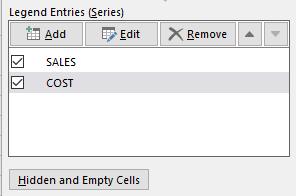
Then click OK to update the chart.
Note: I re-added the data series for Costs for the remainder of the tutorial.
Editing Data in a Chart
To edit another data series in your chart, right-click the chart and select Select Data.
The following dialog box will appear.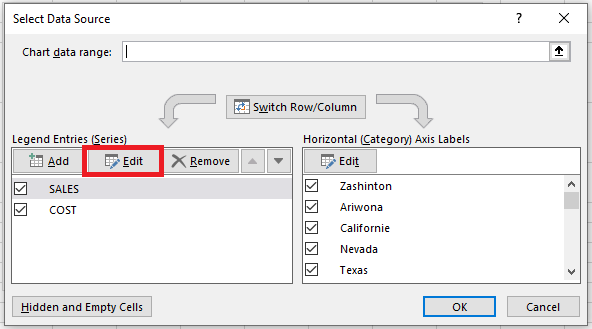
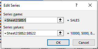
Click the Edit button. The following window will open, allowing you to edit the series name and the referenced data:
Moving Data Series Up/Down
To move a series up or down, select it and then click the up/down arrows to rearrange it.
For example, I will move the Costs data series upward: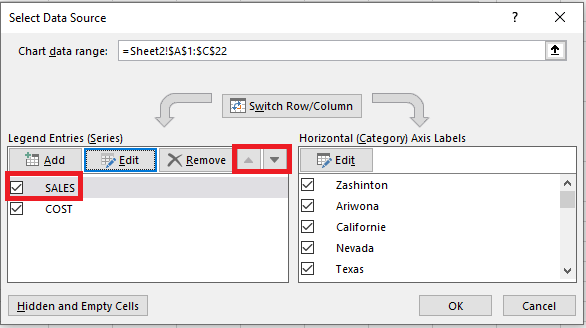
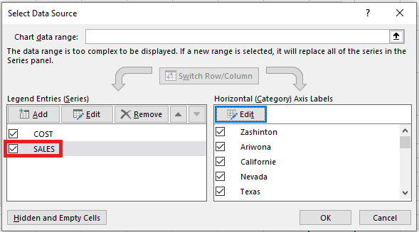
Then click OK to update the chart.
Notice how the bars have reversed order.
Creating a New Chart in Excel
Creating a chart is fairly straightforward:
- Make sure your data is appropriate for a chart.
- Select the range that contains your data.
- Go to the Insert tab and select a chart type from the Charts group. These icons open drop-down lists that display subtypes. Excel creates the chart and places it in the center of the window.
There are three entry points for creating a chart:
- Quick Analysis icon
- Recommended Charts
- Insert tab on the ribbon
Creating a Chart Using the Quick Analysis Icon
When you select a data range in Excel, the Quick Analysis icon appears just below the data.
Clicking it opens a menu with options for formatting, charts, totals, tables, and sparklines.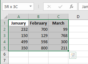
Click the Charts tab and the Quick Analysis tool will display a few recommended charts.
Hover over any thumbnail to see a live preview.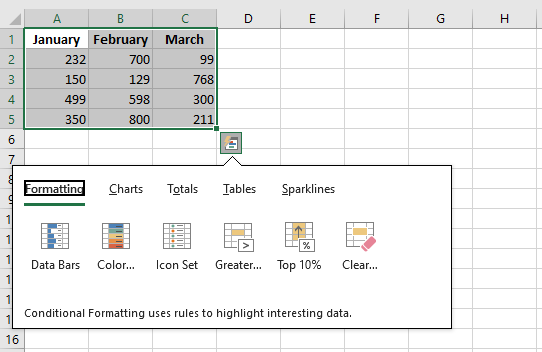
If none of the thumbnails suit your needs, you can click the More Charts icon at the end—equivalent to selecting the Recommended Charts icon.
Although this tool is handy, it often takes at least three clicks and some hovering to access suitable charts. It’s usually easier to go directly to Recommended Charts.
Inserting a Recommended Chart
You’ll likely prefer the Recommended Charts method to create charts.
This icon appears as a large button in the Charts group on the Insert tab.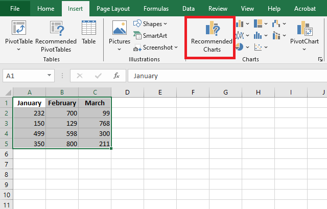
Select your data range and click Recommended Charts.
Excel opens the Insert Chart dialog box, starting with the Recommended Charts tab.
You’ll see chart previews without needing to hover over each one.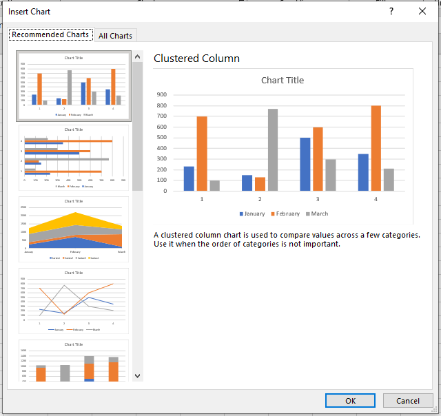
If none of the recommended charts fits your needs, switch to the All Charts tab to browse the 73 built-in chart types.
This tab is easier to navigate than the icons on the ribbon and includes chart types like Surface and Stock, which are hidden from the main ribbon.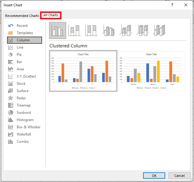
Each category shows thumbnails, typically including:
- Clustered – Displays each series as a separate bar, column, or marker starting from the axis.
- Stacked – Shows how series add up to a total. Good for total sales by region, less useful for analyzing individual series trends.
- 100% Stacked – Converts values into percentages; each bar/line/column totals 100%. Not ideal for comparing raw values.
- 3D Column – Adds depth by showing series front to back. May obscure data if front series are taller than the back.
Creating a Chart Using Other Insert Icons
If you don’t use the Recommended Charts icon, you can directly access one of the eight other chart type dropdowns in the Insert tab.
There are 11 chart categories, but only eight icons are visible.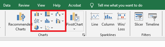
- Bubble charts are found under the Scatter chart icon.
- Stock and Surface charts are under the Radar icon.
- Cone, Pyramid, and Cylinder options were moved to the Format Pane.
To access chart templates or recently used charts, go to Insert Chart → All Charts.
NOTE
You can create a chart with a single keystroke. Select the range you want to use in the chart, and then press Alt+F1 (for an embedded chart) or F11 (for a chart on a chart sheet). Excel displays the chart of the selected data using the default chart type. The default chart type is a column chart, but you can change it. To change the default chart type, select any chart and choose Chart Tools / Design / Change Chart Type. The Change Chart Type dialog box appears. Choose a chart type from the list on the left, then right-click a chart in the row of thumbnails and choose Set as Default Chart.Exploring Other Chart Types
Although a clustered column chart might work well, it’s worth trying other chart types.
Choose:
Chart Tools → Design → Change Chart Type → All ChartsTo change the default chart type:
- Select any chart
- Go to Chart Tools → Design → Change Chart Type
- In the dialog box, right-click a chart thumbnail and choose Set as Default Chart.
The dialog displays a preview of each chart for both data orientations. Click OK to apply your selection.
NOTE:
Chart styles shown depend on the workbook theme. Changing the theme via Page Layout → Themes alters available styles and colors.
Working with Charts
This section covers common chart tasks:
■ Resizing and Moving Charts
- To resize: Click the chart. Drag a corner handle when the pointer becomes a double arrow.
- Alternatively, select the chart, go to Chart Tools → Format → Size, and adjust the Height and Width fields.
- To move: Click and drag the chart’s border.
- To move it to another sheet or workbook, use Cut (Ctrl+X) and Paste (Ctrl+V).
To move between embedded and chart sheet:
Chart Tools → Design → Move Chart■ Copying Charts
To duplicate a chart on the same sheet:
- Ctrl+drag the chart’s border.
To copy a chart to another location or workbook:
- Use Copy (Ctrl+C) and Paste (Ctrl+V).
Charts pasted in another workbook remain linked to their original data.
■ Deleting Charts
To delete an embedded chart:
- Ctrl+click to select it, then press Delete.
- You can select multiple charts with Ctrl+Click.
To delete a chart sheet:
- Right-click the sheet tab → Delete
■ Adding Chart Elements
Click the chart to activate it, then use the Chart Elements (+) icon to add elements like:
- Titles
- Legends
- Data Labels
- Gridlines
Or use:
Chart Tools → Design → Add Chart Element■ Moving and Deleting Chart Elements
To move items like titles or legends:
- Click and drag their border.
To delete:
- Select the item and press Delete, or use the Chart Elements (+) menu.
■ Printing Charts
Embedded charts print like any other worksheet content.
Use Print Preview or Page Layout view to avoid page breaks splitting your chart.Charts on chart sheets always print one per page.
To exclude a chart from printing:
- Open Format Chart Area pane → Size & Properties → uncheck Print Object
NOTE:
If you select an embedded chart and go to File → Print, Excel prints the chart by itself—not the entire worksheet.
Understanding Chart Types
Charts are typically used to support a message or highlight a point. That message may appear in the title or a textbox.
Choosing the right chart type is key. It’s often worth testing several chart types to find the most effective one.
Underlying most charts is a comparison, such as:- Item comparison: Sales by region
- Time comparison: Sales over months
- Relative comparison: Pie charts for percentages
- Relationship comparison: XY scatter plot
- Frequency comparison: Histogram of grade distribution
- Outlier detection: Large datasets revealing anomalies
Choosing a Chart Type
A common question is:
“How do I know which chart type to use?”There’s no one-size-fits-all answer. The best advice:
Use the chart type that communicates your message most clearly.Recommended Charts is a good starting point:
Insert → Charts → Recommended ChartsOn the ribbon, the Charts group offers nine dropdowns, each giving access to multiple types (e.g., column/bar under one button, scatter/bubble under another).
The All Charts tab in the Insert Chart dialog box shows a categorized list of all types and subtypes.
Choosing a Chart Type
A common question among Excel users is: “How do I know which chart type to use for my data?” Unfortunately, there’s no one-size-fits-all answer. The best advice is probably vague: use the chart type that conveys your message most clearly. Excel’s Recommended Charts feature is a good starting point. Select your data and choose Insert > Charts > Recommended Charts to see the types Excel suggests. Keep in mind, though, that these suggestions are not always the best choice.
In the ribbon, the Charts group on the Insert tab displays the Recommended Charts button, along with nine other dropdown buttons. Each of these dropdowns contains multiple chart types. For example, column and bar charts are accessed from a single dropdown, as are scatter and bubble charts. The easiest way to pick a specific chart type is probably to select Insert > Charts > Recommended Charts, which opens the Insert Chart dialog box. Select the All Charts tab to get a concise list of all chart types and their subtypes.
Column Charts
The most common chart type is probably the column chart, which displays each data point as a vertical column, with the height representing the value. The value axis is shown vertically, typically on the left side of the chart. You can include any number of data series, and data points in each series can be stacked. Typically, each data series is displayed in a different color or pattern.
Column charts are often used to compare discrete items and can show differences between elements within a series or across multiple series. Excel offers seven column chart subtypes.
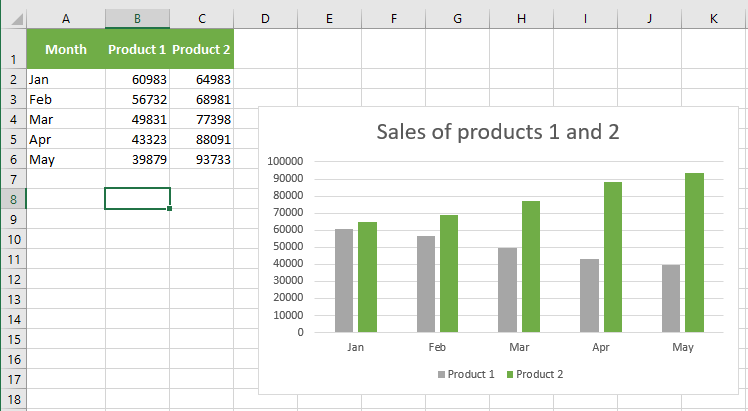
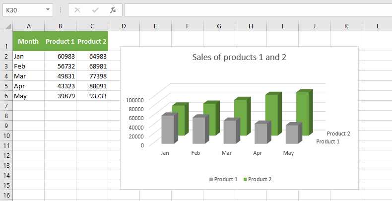
The following figure shows an example of a clustered column chart representing monthly sales of two products.
From this chart, it’s clear that Product 1 consistently outsold Product 2. Also, sales of Product 2 declined over the five-month period, while sales of Product 1 increased.
The same data is shown in the next figure as a stacked column chart.
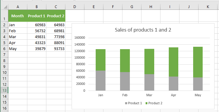
This chart has the added benefit of displaying combined sales over time. It shows that total sales remained fairly steady each month, but the relative proportions of the two products shifted.
A 100% stacked column chart of the same data appears in the next figure.
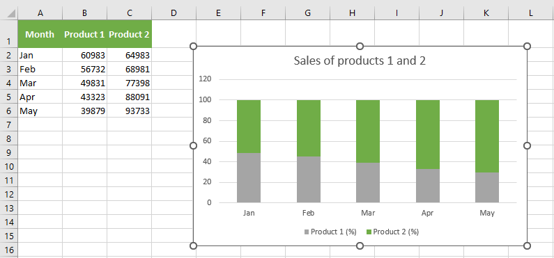
This chart highlights each product’s relative contribution by month. Note that the vertical axis displays percentages, not actual sales amounts. This chart provides no information about total sales volume, though that could be added using data labels. This type of chart is often a good alternative to multiple pie charts. Rather than using a pie for each year to show relative sales volume, this chart uses one column per year.
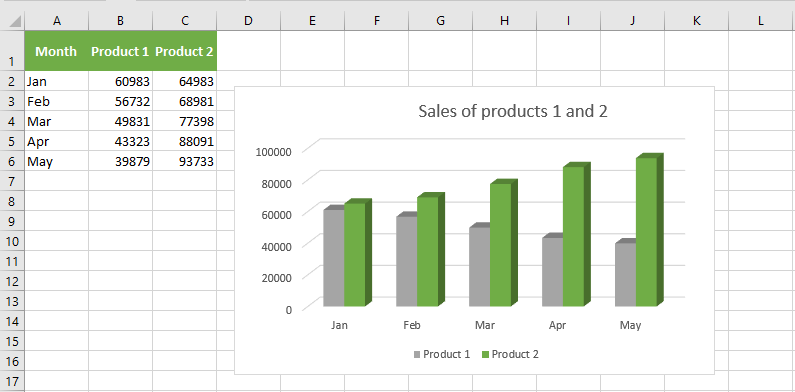
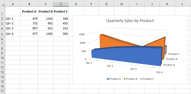
The next figure displays the same data as a 3-D clustered column chart.
The name is a bit misleading, as the chart only uses two dimensions. Many people use this chart type for its visual appeal. Compare it to a “true” 3-D column chart (with a second category axis), as shown in the next figure.
This chart may be visually striking, but precise comparisons are difficult due to the distorted perspective.
For 3-D columns, you can choose a different column shape in the Format Data Series dialog box. Excel offers variants such as cylinder, cone, and pyramid.
Bar Charts
A bar chart is essentially a column chart rotated 90 degrees clockwise. One advantage of bar charts is that category labels are often easier to read. The next figure shows a bar chart displaying one value for each of ten survey items.
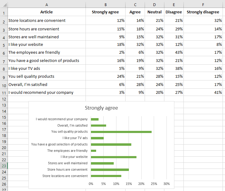
The category labels are long and would be hard to read clearly on a column chart. Excel provides six bar chart subtypes.
Unlike column charts, no bar chart subtypes display multiple series along a third axis (i.e., Excel does not offer 3-D bar chart subtypes). You can add a 3-D effect to a bar chart, but it will still use only two axes.
You can include any number of data series in a bar chart. Also, bars can be “stacked” from left to right.
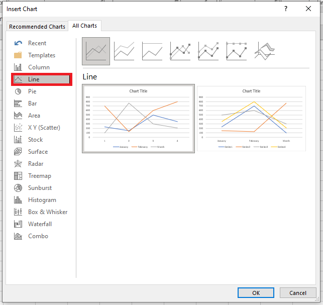
Line Charts
Line charts are often used to plot continuous data and are useful for identifying trends. For example, plotting daily sales as a line chart may help you spot fluctuations over time. Typically, the x-axis of a line chart displays evenly spaced intervals. Excel supports seven line chart subtypes.
See the next figure for an example of a line chart that plots monthly data (676 data points).
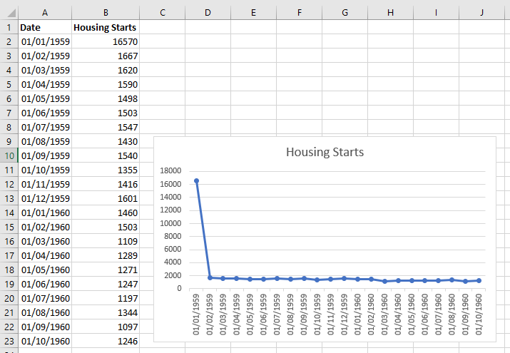
Although the data varies significantly month-to-month, the chart clearly outlines cycles.
A line chart can use any number of data series. You distinguish the lines using different colors, line styles, or markers. The next figure shows a line chart with three series.
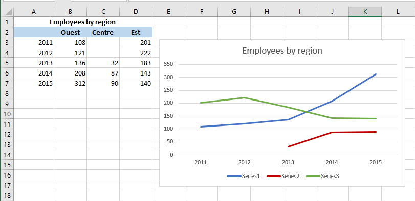
Series are differentiated using markers (circles, squares, triangles) and line colors. When printed in black and white, markers are the only way to distinguish the lines.
The final example, shown in the next figure, is a 3-D line chart.
Although visually appealing, it’s certainly not the clearest way to present data—in fact, it’s quite poor.
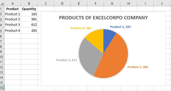
Pie Charts
A pie chart is useful when you want to show relative proportions or contributions to a whole. A pie chart uses a single data series. Pie charts are most effective with a small number of data points. As a general rule, a pie chart should not use more than five or six data points (or slices). A pie chart with too many data points can be difficult to interpret.
All values in a pie chart must be positive numbers. If you create a pie chart using one or more negative values, the negative values will be converted to positive values, which is likely not what you intended.
You can « explode » one or more slices in a pie chart to emphasize them. Activate the chart and click on any slice to select the whole pie. Then click again on the slice you want to explode and drag it away from the center.
XY (Scatter) Charts
Another common chart type is the XY chart (also called a scatter chart). An XY chart differs from most other chart types in that both axes display values.
This chart type is often used to show the relationship between two variables.
The following figure shows an example of an XY chart that plots the relationship between sales calls made (horizontal axis) and sales (vertical axis).
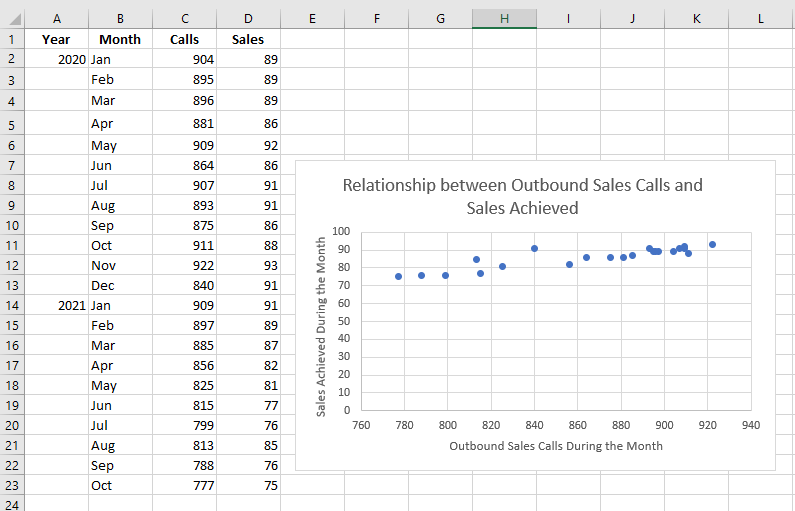
Each point on the chart represents a month. The chart shows that these two variables are positively correlated: months with more sales calls generally had higher sales volumes.
Although the data points relate to time, the chart doesn’t convey any time-related information. In other words, the points are plotted based solely on their two values.
Area Charts
Think of an area chart as a line chart where the area beneath the line is filled with color. The following figure shows an example of a stacked area chart.
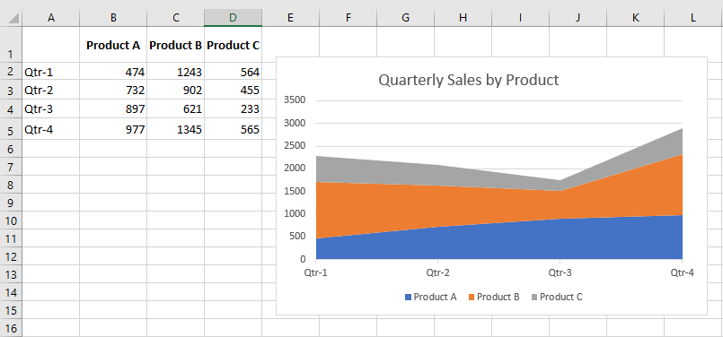
Stacking data series makes it easy to see the total as well as the contribution of each series.
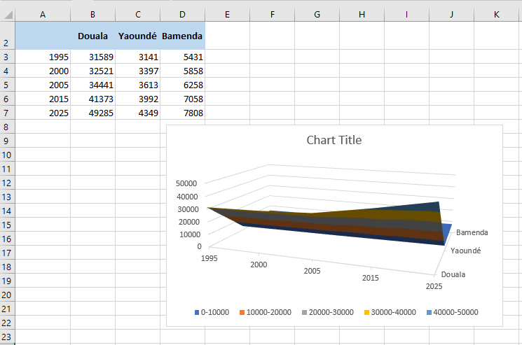
The next figure shows the same data plotted as a 3-D area chart.
As you can see, this is not an effective chart. The data for Products B and C is obscured. In some cases, rotating the chart or using transparency may solve the problem. But generally, the best solution is to select a different chart type.
Radar Charts
You may not be familiar with this chart type. A radar chart is a specialized chart that has a separate axis for each category, and the axes extend outward from the center of the chart. The value of each data point is plotted on the corresponding axis.
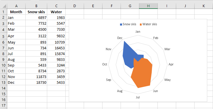
This chart displays two data series across 12 categories (months) and illustrates the seasonal demand for snow skis versus water skis. Note that the water ski series partially obscures the snow ski series.
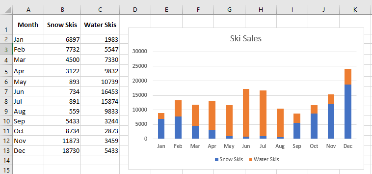
Using a radar chart to display seasonal sales can be visually interesting, but it’s certainly not the most effective chart type. As shown in the next figure, a stacked bar chart communicates the information much more clearly.
Surface Charts
Surface charts display at least two data series on a surface. As shown in the following figure, these charts can be quite eye-catching.
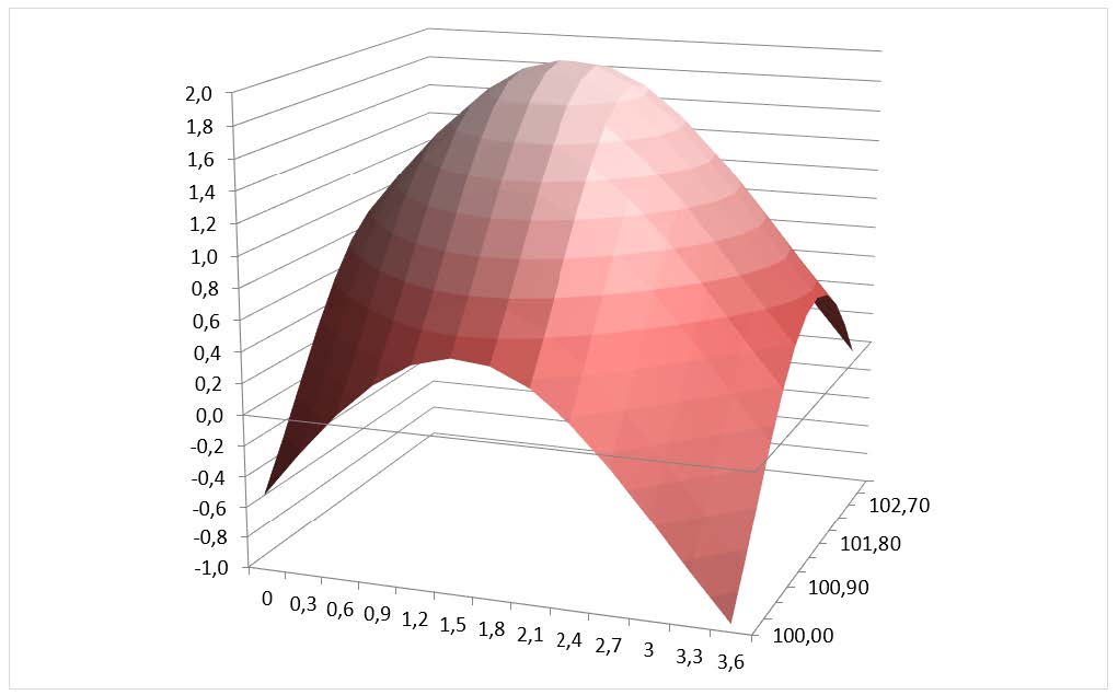
Unlike other charts, Excel uses color to distinguish values—not data series. The number of colors used is determined by the major unit setting on the value axis scale. Each color corresponds to one major unit.
NOTE:
A surface chart does not plot true 3-D data points. The series axis for a surface chart, like all other 3-D charts, is a category axis, not a value axis. In other words, if you have data represented by x, y, and z coordinates, it cannot be plotted accurately on a surface chart unless the x and y values are equally spaced.
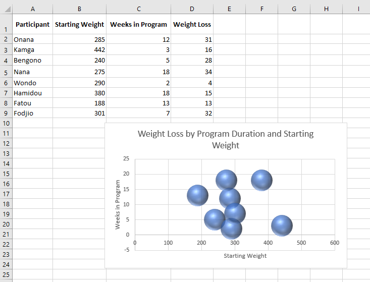
Bubble Charts
A bubble chart is essentially an XY chart that can display an additional data series represented by bubble size. Like an XY chart, both axes are value axes (there is no category axis).
The following figure shows an example of a bubble chart illustrating the results of a weight loss program. The horizontal axis represents initial weight, the vertical axis shows the number of weeks in the program, and the size of the bubble represents the amount of weight lost.
Stock Charts
Stock charts are most useful for displaying stock market data. These charts require three to five data series, depending on the subtype.
The figure below shows an example of each of the four stock chart types.
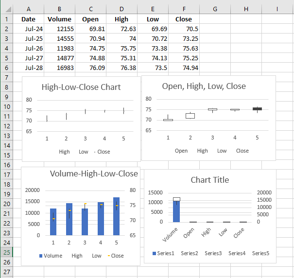
The two bottom charts display trading volume and use two value axes. Daily volume, shown as columns, uses the left axis. The vertical bars (sometimes called candlesticks) represent the difference between opening and closing prices. A black bar indicates the closing price was lower than the opening price.
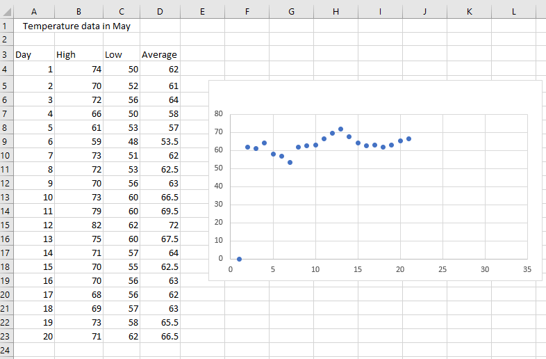
Stock charts aren’t limited to stock price data. The following figure shows a stock chart depicting daily high, low, and average temperatures for each day in May. This is a high-low-close chart.
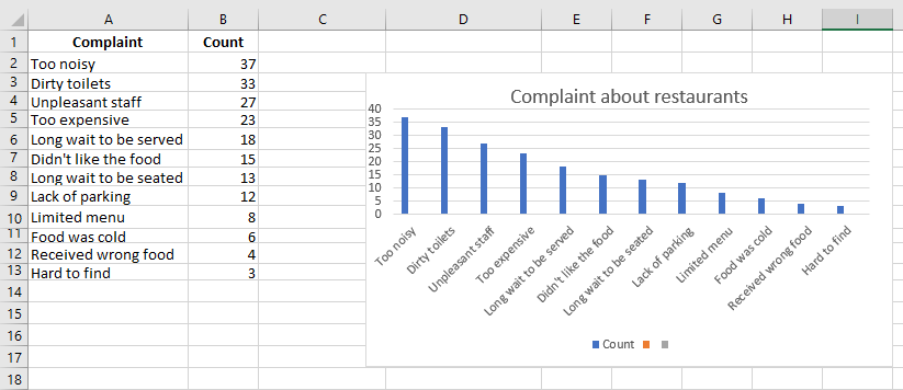
Pareto Charts
A Pareto chart is a combination chart in which columns are displayed in descending order and use the left axis. The line shows the cumulative percentage and uses the right axis.
The figure below shows a Pareto chart created from the data in range A2:B14. Note that Excel sorted the chart items. The line shows, for example, that about 50 percent of all complaints fall into the first three categories.
Waterfall Charts
A waterfall chart is used to show the cumulative effect of a series of numbers, typically including both positive and negative values. The result is a “staircase” style visual.
The following figure shows a waterfall chart based on the data in column D.
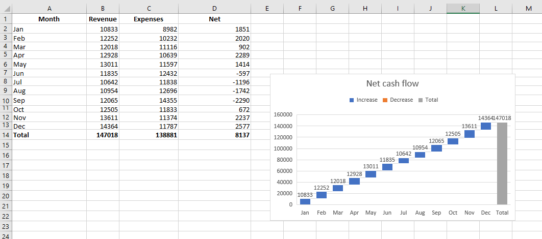
Waterfall charts typically display the final total as the last column, starting from zero. To correctly display the total column, select it, right-click, and choose Set as Total from the context menu.
Box and Whisker Charts
A box and whisker chart (also called a quartile chart) is often used to visually summarize data. In the past, such charts could be created in Excel, but doing so required a lot of setup. In recent versions of Excel, it’s simple.
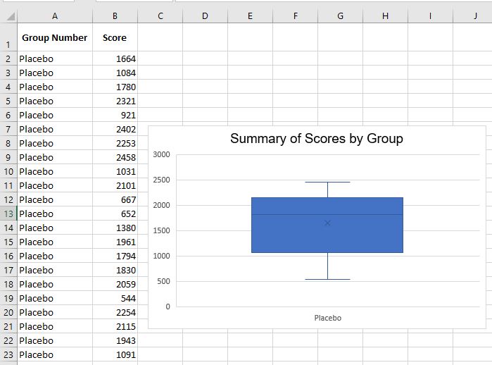
The data is in a two-column table. In the chart, the vertical lines extending from the box represent the numerical range (minimum and maximum values). The “box” represents the 25th to 75th percentile. The horizontal line within the box is the median (50th percentile), and the X represents the mean. This chart type allows quick comparisons between data groups.
As shown in the figure, the Series Options section of the Format Data Series pane contains specific settings for this chart type.
Sunburst Charts
A sunburst chart is like a multi-layered pie chart. This type of chart is particularly useful for hierarchically structured data. The figure below shows a sunburst chart representing a music collection.
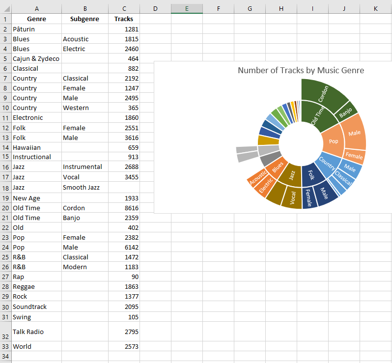
It displays the number of tracks per genre and subgenre. Note that some genres do not have subgenres.
A potential issue with this chart type is that some slices are too small for data labels to be displayed.
Treemap Charts
Like a sunburst chart, a treemap chart is suited for hierarchical data. However, the data is displayed as rectangles. The figure below shows the same example data as a treemap chart.
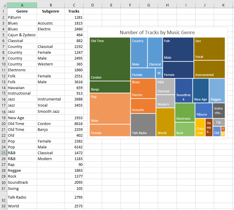
Chart Sheets in Excel
When a chart is placed on a chart sheet, you can view it by clicking on its sheet tab. A chart sheet contains only a single chart (and no cells). Chart sheets and worksheets can be interspersed within a workbook.
To move an embedded chart to a chart sheet, click the chart to select it, then go to:
Chart Tools → Design → Location → Move Chart.
The Move Chart dialog box, shown in the figure, will appear. Select the New sheet option and assign a name to the chart sheet (or accept Excel’s default name). Click OK, and the chart is moved, and the new chart sheet becomes active.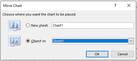
The Move Chart dialog box allows you to move a chart to a chart sheet.
NOTE:
This process also works in reverse: you can select a chart on a chart sheet and move it back to a worksheet as an embedded chart. In the Move Chart dialog box, choose Object in, then select the worksheet from the dropdown list.
When you place a chart on a chart sheet, it occupies the entire sheet.
If you plan to print a chart on a page by itself, using a chart sheet is often your best option.
If you have many charts, you can place each one on a separate chart sheet to avoid cluttering your worksheet.
This technique also makes it easier to locate a specific chart, as you can rename the sheet tabs to reflect the contents of each chart.Embedded Charts in Excel
An embedded chart essentially floats above a worksheet, on the worksheet’s drawing layer. The chart shown earlier is an example of an embedded chart.
Just like other drawing objects (such as Shapes or SmartArt), you can move an embedded chart, resize it, change its proportions, adjust its borders, and perform various other operations.
Using embedded charts allows you to print the chart alongside the data it is based on.To make changes to the actual chart within an embedded chart object, you must click the chart to activate it. When a chart is activated, Excel displays the Chart Tools contextual tab.
The ribbon provides many tools for working with charts, and even more tools are available in the Format task pane.With one exception, every chart starts as an embedded chart. The exception is when you create a default chart by selecting data and pressing F11. In that case, Excel creates the chart on a separate chart sheet.
Understanding How Excel Handles Charts in Excel
Before you can create a chart, you must have data. The data is stored in cells within a worksheet. Typically, the data used for a chart resides on a single worksheet, but this is not a strict requirement. A chart can use data stored on another worksheet—or even in a different workbook.
A chart is essentially an object that Excel creates on demand. This object consists of one or more data series that are graphically displayed. The appearance of each data series depends on the selected chart type.
For example, if you create a line chart that uses two data series, the chart will contain two lines—each representing one of the series. The data for each series is stored in a separate row or column. Each point on the line is determined by the value in a single cell and is represented by a data marker. You can distinguish each line by its thickness, line style, color, or data markers.A key point to keep in mind is that charts are dynamic. In other words, a chart series is linked to your worksheet data. If the data changes, the chart is automatically updated to reflect those changes.
After creating a chart, you can always modify its type, adjust formatting, add or remove specific elements (such as the title or legend), add new data series, or change an existing series to reference a different range of data.
A chart is either embedded in a worksheet or displayed on a separate chart sheet. It’s easy to move an embedded chart to a chart sheet—and vice versa.