Étiquette : practical-excel

Two of the most useful yet simple functions provided by Microsoft Excel are the MIN and MAX functions. The MAX function in Excel allows you to find the highest numeric value within a range of cells. Its opposite, the MIN function, returns the lowest numeric value in a given range. One advantage of these functions is that they can be combined with other functions such as IF.

Using the MAX Function to Determine the Highest Value in a Range
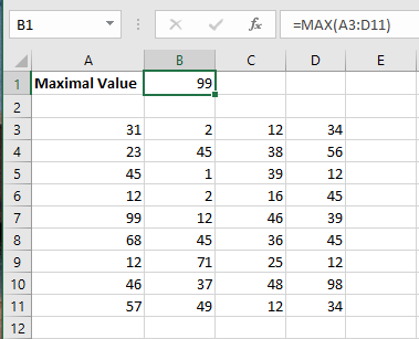
This example finds the highest value in the range A3:D11 using the MAX function. The return value of the function is the maximum value in the set.
=MAX(number1, number2, …)
number1, number2, …: Between 1 and 30 numbers for which you want to find the largest value. You can use cell references; however, the cells must contain numbers or values that can be converted into numbers.

To determine the maximum value:

• In cells A3:D11, enter a series of values.
• In cell B1, type the formula:
  =MAX(A3:D11)
• Press Enter.

Using the MIN Function to Find the Employee with the Lowest Sales
In a company, employee sales are monitored. Columns B to E contain sales figures for the first four months of the year. To find out which employee has the lowest monthly sales, use the MIN function. The return value of the function is the smallest number in a set.
=MIN(number1, number2, …)
number1, number2, …: Between 1 and 30 numbers for which you want to find the smallest value. You can use cell references; however, the cells must contain numbers or values that can be converted into numbers.

Using the MIN Function to Detect the Smallest Value in a Column
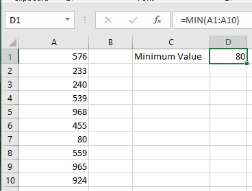
To determine the smallest value in a single column, use the MIN function. The function returns the lowest value in a set. The syntax is the same as described in the previous example.

To determine the minimum value in a column:

• In column A, enter any value into cell A10.
• Select cell B1 and type the following formula:
  =MIN(A1:A10)
• Press Enter.

Using the SUM Function to Add a Range
The SUM function is used in Excel to add a range of cells, an entire column, or non-contiguous cells. As part of the Math & Trigonometry category, it is entered by typing “=SUM()” followed by the values to be added. The values provided to the function can be numbers, cell references, or ranges.
For example, cells B1, B2, and B3 contain 20, 44, and 67 respectively. The formula « =SUM(B1:B3) » adds the numbers in cells B1 to B3 and returns 131. The SUM formula automatically updates when a value is inserted or deleted. It also includes any changes made to an existing range of cells. Moreover, the function ignores empty cells and text values. The syntax is:
=SUM(number1, [number2], [number3], …)

The SUM function uses the following arguments:
■ Number1 (required) – This is the first item you want to add.
■ Number2 (required) – The second item you want to add.
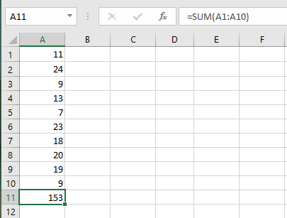
■ Number3 (optional) – The third item you want to add.

In this example, all values in a range on a worksheet need to be added, with the total displayed in cell A11. To do this, use the SUM function, which returns the sum of all numbers in a range of cells.

To sum a range:

• In cells A2:A10, enter any value between 1 and 100.
• In cell A11, type the following formula:
  =SUM(A2:A10)
• Press Enter.

Using the SUM Function to Add Multiple Ranges
NOTE:
To perform this task more quickly, simply select cell A11 and click the Σ (AutoSum) icon in the editing bar under the Home tab. Then press Enter to display the result.

To add multiple ranges, just refer to each one, separated by semicolons, using the SUM function.

To add multiple ranges:

• In cells A2:A10, enter amounts ranging from 1 to 100.
• Select cells B2:B10 and type the formula =A2*8% to calculate the tax amount.
• Press Ctrl+Enter.
• In cells D2:D10, enter discount values from –1 to –3.
• In cell B12, add the three columns using the following function:
  =SUM(A2:A10, B2:B10, D2:D10)
• Press Enter.

Summing an Entire Column
You can also use the SUM function in Excel to add an entire column.

NOTE:
To place a border around all cells used in the function, select cell B12 and press F2. The function will also be displayed.

You can also use the SUM function in Excel to add an entire row. For example, =SUM(5:5) adds all the values in row 5.

Summing Non-Contiguous Cells
You can also use the SUM function in Excel to add non-contiguous cells. Non-contiguous means they are not adjacent to each other.

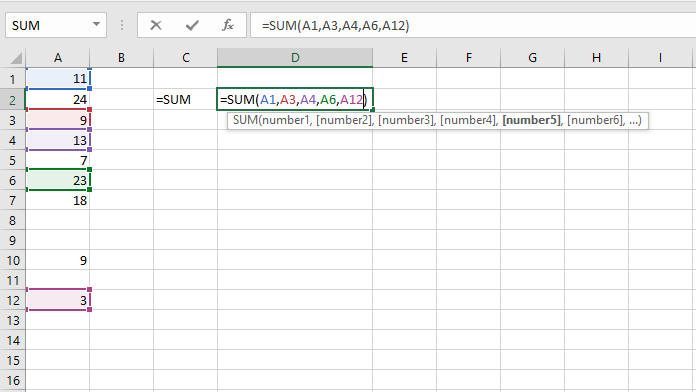
Note: =A2+A4+A5+A7+A13 produces exactly the same result!

AutoSum
Use AutoSum or press ALT + = to quickly sum a column or row of numbers.

• First, select the cell below the column of numbers (or next to the row of numbers) you want to sum.

• Under the Home tab, in the Editing group, click AutoSum (or press ALT + =).

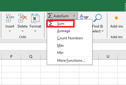
• Press Enter.

Here’s a very simple and concise definition of a circular reference provided by Microsoft:
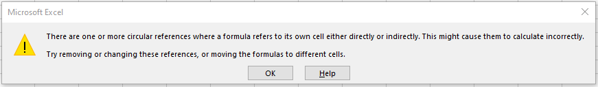
« When an Excel formula refers to its own cell, either directly or indirectly, it creates a circular reference. »

For example, if you select cell A1 and type =A1, that creates a circular reference in Excel.
Typing any other formula that refers to A1, such as =A1*5 or =IF(A1=1, "OK", ""), would have the same effect.

As soon as you press Enter to complete such a formula, you’ll see the following warning message:

Why Does Excel Warn You?

Because circular references can cause infinite loops, slowing down your workbook’s calculations significantly.

After you receive the warning, you can click Help for more info or close the message window by clicking OK or the X button.
Once the window is closed, Excel displays either zero (0) or the last successfully calculated value in the cell.

In some cases, a formula with a circular reference may complete successfully before it begins recalculating, and when that happens, Excel returns the last known valid value.

When you enter multiple formulas with circular references, Excel doesn’t always show the warning repeatedly.

But Why Would Anyone Create Such a Problematic Formula?

Sometimes, you may accidentally create a circular reference. Here’s a very common scenario:
Suppose you want to sum the values in column A using the SUM function, and you inadvertently include the total cell itself (e.g., B6) in the sum range.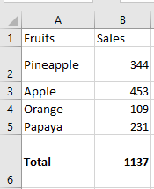

If circular references are not allowed in your Excel (they’re disabled by default), you’ll see an error message.
If iterative calculations are enabled, your circular formula will return 0, as shown above.

Sometimes, blue arrows may also suddenly appear in your worksheet, making it look like Excel is acting up.

Actually, these arrows are just Trace Precedents or Trace Dependents tools that indicate which cells influence or are influenced by the active cell.

Are Circular References Always Bad?

At this point, you may feel like circular references are completely useless and dangerous, and wonder why Excel allows them at all.

However, there are rare cases where a circular reference can provide a shorter and more elegant solution.

Example: Using a Circular Reference in Excel

Suppose you have a list of items in column A, and you enter a delivery status in column B.
As soon as you type “Yes” in column B, you want the current date and time to be automatically entered in column C on the same row — as a static, unchanging timestamp.

Using the NOW() function isn’t an option because it’s volatile and updates every time the sheet is recalculated.

A better solution is to use nested IF functions with a circular reference like this:=IF(B3="YES", IF(C3="", NOW(), C3), "")


Where B3 is the delivery status and C3 is where the timestamp appears.

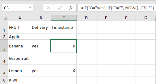
In this formula, the first IF checks cell B3 for “YES” and, if true, runs the second IF.
If false, it returns an empty string.
The second IF is a circular formula that captures the current date and time only if C3 is empty — preserving all existing timestamps.

Note:
For this formula to work, you must enable iterative calculations in your worksheet — which we’ll cover next.

How to Enable/Disable Circular References

As mentioned, iterative calculations are turned off by default in Excel.
(Iteration means repeated recalculation until a specific numeric condition is met.)

To enable circular formulas to function, you need to activate iterative calculation in your workbook.

In Excel 2019, 2016, 2013, or 2010:

• Go to File > Options
• Select Formulas
• Check the box Enable iterative calculation under Calculation options

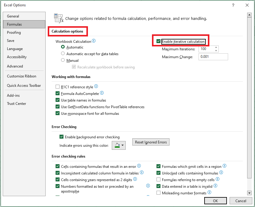
When you enable iterative calculation, you must define two settings:
■ Maximum Iterations – The number of times a formula should recalculate. Higher numbers slow down performance.
■ Maximum Change – The minimum amount of change between calculation results. Smaller numbers improve accuracy but increase time.

The default settings are:

• Maximum Iterations: 100
• Maximum Change: 0.001

This means Excel will stop recalculating your circular formula after 100 iterations or when the result changes by less than 0.001, whichever comes first.

Why You Should Avoid Circular References

As you’ve seen, circular references are generally a risky and discouraged practice in Excel.

In addition to:

• Slower performance
• Warning messages every time the workbook opens (unless iteration is enabled)
  They may also create invisible problems.

For example, if you:

• Select a cell with a circular reference
• Accidentally press F2 (Edit mode)
• And press Enter without making changes
  → The formula will recalculate and return 0.

Tip from Excel experts:
Avoid circular references as much as possible in your worksheets.

How to Find Circular References in Excel

To locate circular references in your workbook:

• Go to the Formulas tab
• Click the arrow next to Error Checking, then hover over Circular References
• The last circular reference entered will be listed

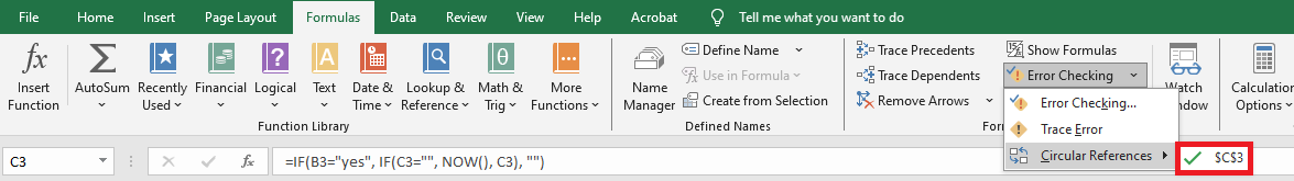
• Click the listed cell and Excel will take you directly to it.
  The status bar will show a message indicating circular references were found and display the address of one such cell.

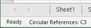
Note:
If circular references exist in another sheet, the status bar will only display “Circular References” without a cell address.
This feature is disabled when iterative calculation is turned on, so you must disable it first to locate circular references.

How to Remove Circular References

Unfortunately, Excel does not offer a one-click solution to remove all circular references in a workbook.

You need to:

• Inspect each circular reference manually (as shown above)
• Either delete the formula
• Or replace it with one or more simpler, non-circular formulas

How to Trace Relationships Between Formulas and Cells

When a circular reference isn’t obvious, the Trace Precedents and Trace Dependents tools can help.
They draw lines showing which cells affect or are affected by the selected cell.

To view these arrows:

• Go to the Formulas tab
• In the Formula Auditing group, click:
• Trace Precedents – Shows which cells provide data to the formula (i.e., which cells influence the selected cell)
• Trace Dependents – Shows which cells depend on the selected cell (i.e., which formulas refer to it)

To hide the arrows, click Remove Arrows (located under Trace Dependents).

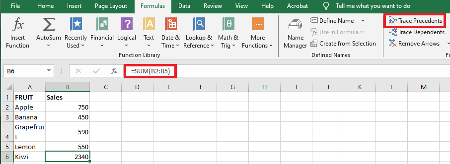
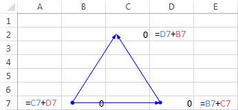
In the example above, the Trace Precedents arrow shows which cells feed into B6.
As you can see, B6 is included in its own formula, creating a circular reference that returns zero.

This case is easy to fix—simply replace B6 with B5 in the SUM argument:=SUM(B2:B5)


Other circular references might not be so obvious and require more thought and calculation.

If a cell contains a formula whose result will never change, you can convert the formula into its static value.
This not only speeds up recalculations in large worksheets but also frees up memory, since values use less memory than formulas.
For example, you might have formulas in part of your worksheet that use values from a previous fiscal year.
Since those numbers are unlikely to change, you can safely convert the formulas to their values.

To do this, follow these steps:

• Select the cell containing the formula you want to convert.
• Double-click the cell or press F2 to enter Edit mode.
• Press F9. The formula is replaced with its result.
• Press Enter or click the Enter button. Excel replaces the formula with the calculated value.

You will often need to use the result of a formula in multiple locations.
For example, if a formula is in cell C5, you can display its result in other cells by entering =C5 in each of them.

This is the best method if the formula result might change, since Excel automatically updates the dependent cells.
However, if you are sure the result will not change, you can copy only the value of the formula into the other cells.

To do this, follow these steps:

• Select the cell that contains the formula.
• Copy the cell.
• Select the cell or cells where you want to paste the value.
• On the Home tab, open the Paste dropdown list and select Paste Values.
  Excel pastes the value of the original cell into each selected cell.

An alternative method (available since Excel 2003) is to copy the cell, paste it into the destination, click the Paste Options dropdown, and then select Values Only.

Unlike copying a formula, Excel does not adjust cell references when a formula is moved.
There are two ways to move a formula in Excel: using the Cut and Paste commands, or by dragging and dropping the formula to its new location.

To drag and drop a formula:

• Select the range D4:D10.
• Position your mouse pointer on the edge of the selected range; when it turns into a four-headed arrow, click and drag the selection to cell E4.
• Release the mouse button to drop the range in its new location.

Quickly move a range of cells to a new location with a simple click and drag-and-drop.

To move a formula using Cut and Paste:

• Select the range E4:E10.
• On the Home tab, click Cut. A blinking dashed border will appear around the selected range.
• Click cell D4, then on the Home tab, click Paste.
  Excel pastes the selected range in the new location.

After creating a formula in Excel, you can use the Copy and Paste commands to duplicate or move the formula to other areas of your worksheet.
When you copy formulas that contain cell references, Excel automatically adjusts those references relative to their new location—unless you specify otherwise.

Using Absolute and Relative Cell References

When you use cell references in your formulas, Excel uses the data stored in those locations for calculations.
The benefit is that if you change the source data, the formula result also updates.

If you copy a formula from one place to another, Excel adjusts the cell references based on the new location.
For example, the formula =B2*B3 entered in cell B5 would become =C2*C3 when copied to cell C5.

However, you can change a reference so that it always points to the original location.
An absolute cell reference remains fixed even when copied or moved.
A relative cell reference adjusts to its new location.
The dollar sign ($) is used to indicate that part of a reference should remain fixed.
Use the dollar sign to specify whether the row, column, or both should be locked.

Examples of Absolute and Relative References in Excel:

Cell Reference	Meaning
$A6	Column A stays fixed, row 6 adjusts
A$6	Row 6 stays fixed, column A adjusts
$A$6	Both column A and row 6 stay fixed
A6	Both column and row adjust to the new position

Making a Cell Reference Absolute in Excel

The following example shows how to make a cell reference absolute:

• Type = in cell D5.
• Point to cell B5, then press the F4 key on your keyboard.
  Excel inserts dollar signs ($) in the reference to make it absolute.
• Type +, then point to cell C5.
• Press Enter.
  The resulting formula in cell D5 will now be: =$B$5+C5.

Copying Formulas with AutoFill

The AutoFill feature allows you to quickly copy a formula to adjacent cells.
Follow these steps to practice using AutoFill:

• Click in cell D5.
• On the Formulas tab, choose AutoSum.
  Excel adds the values from the adjacent cells, which in this case are B5:C5.
  Press Enter.
• Click cell D5, then drag the AutoFill handle down to cell D9 and release.
  Excel copies the formula from D5 and adjusts the cell references accordingly.

NOTE:
When you use a named range in a formula, Excel automatically treats the reference as absolute.
In other words, when you copy a formula that uses a named range, the reference does not change based on location.

The AutoFill feature allows you to quickly copy a formula into adjacent cells.

Copying Formulas with Copy and Paste

When you use the Copy command, Excel stores a copy of the selection in the clipboard, allowing you to paste the data multiple times.
Follow these steps to practice copying and pasting formulas:

• Click cell B10.
• On the Home tab, in the Clipboard group, click Copy.
• Select the range C10:D10.
• In the Clipboard group, click Paste.
  Excel pastes the formula from cell B10 and adjusts the references accordingly.

Pasting Formula Results in Excel

With the Paste Values command, you can copy a formula and paste only its result into another cell.
Follow these steps to practice pasting formula results:

• Select cell H8 and choose Copy from the Home tab.

NOTE:
You can also press the Enter key to paste into a worksheet cell,
but doing so removes the item from the clipboard.

• Click cell I8, then on the Home tab, choose Paste and select Paste Special.
  The Paste Special dialog box appears.
• In the dialog box, select Values and click OK.

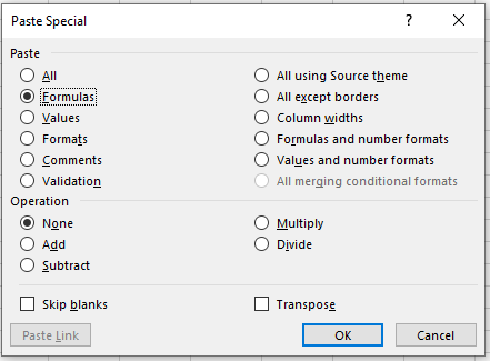
Paste the results of formulas into a separate cell.

Entering a new formula in a worksheet seems like a simple process:

• Select the cell where you want to enter the formula.
• Type an equal sign (=) to tell Excel you’re entering a formula.
• Enter the operands and operators for the formula.
• Press Enter to confirm the formula.

After entering a formula, you may need to go back and make changes. Excel offers three methods to enter Edit mode and modify a formula in the selected cell:
■ Press F2
■ Double-click the cell
■ Use the Formula Bar to click anywhere within the formula text

Excel categorizes formulas into four groups: arithmetic, comparison, text, and reference. Each group has its own set of operators, and each is used in different ways. The following sections explain how to use each type of formula.

Using Arithmetic Formulas

Arithmetic formulas are by far the most common type. These formulas combine numbers, cell addresses, and function results with mathematical operators to perform calculations.
Table 4.1-a summarizes the mathematical operators used in arithmetic formulas:

Table: Arithmetic Formula Operations

Operator	Name	Example	Result
+	Addition	=5 + 11	16
-	Subtraction	=11 - 5	6
-	Negation	=-5 - 11	-16
*	Multiplication	=10 * 550	5500
/	Division	=15 / 3	5
%	Percentage	=15%	0.15
^	Exponentiation	=10^3	1000

Using Comparison Formulas

A comparison formula is a statement that compares two or more numbers, text strings, cell contents, or function results.
If the statement is true, the formula result is the logical value TRUE, which is equivalent to any non-zero value.
If the statement is false, the formula returns FALSE, which is equivalent to zero.

Table: Comparison Formula Operations

Operator	Name	Example	Result
=	Equal to	=11=6	FALSE
>	Greater than	=11>6	TRUE
<	Less than	=10<5	FALSE
>=	Greater or equal to	="a">="b"	FALSE
<=	Less or equal to	="a"<= "b"	TRUE
<>	Not equal to	="a"<> "b"	TRUE

Comparison formulas have many uses. For example, you can determine whether to pay a sales bonus by comparing actual sales to a predefined quota. If sales exceed the quota, the bonus is awarded.

Using Text Formulas

The arithmetic and comparison formulas discussed earlier calculate or compare values and return results.
However, a text formula is one that returns a text value.
Text formulas use the ampersand operator (&) to work with text cells, quoted text strings, and text function results.

One way to use text formulas is to concatenate text strings. For example, if you enter the formula:
="excel" & "corpo"
Excel will display: excelcorpo.
Note that the quotes and the ampersand do not appear in the result.

Using Reference Formulas

Reference operators combine two cell or range references to create a single reference.
The following table summarizes the operators you can use in reference formulas:

Table: Reference Formula Operations

Operator	Name	Description
:	Range	Creates a range from two cell references, such as A1:D10
(space)	Intersection	Returns a range that is the intersection of two ranges, e.g. A1:D10 B4:F20
,	Union	Returns a range that is the union of two ranges, e.g. A1:D10, B4:F20

Conditional formatting is a powerful feature when it comes to applying different formats to data that meets certain conditions. It helps highlight key information in your worksheets and quickly spot discrepancies in cell values at a glance.

At the same time, conditional formatting is often seen as one of the most complex and obscure Excel functions, especially by beginners. If you feel intimidated by this feature—don’t be! In reality, conditional formatting in Excel is quite simple and easy to use, and you’ll be convinced of that in just 5 minutes after reading this short tutorial.

Basics of Excel Conditional Formatting

Just like standard cell formatting, you use conditional formatting in Excel to style your data by changing fill color, font color, and cell border styles. The difference is that conditional formatting is more flexible—it lets you format only the data that meets specific criteria or conditions.

You can apply conditional formatting to one or more cells, rows, columns, or entire tables based on the content of the cell itself or based on the value of another cell. To do this, you create rules, which define when and how the selected cells should be formatted.

To get started, here’s where to find the conditional formatting feature in various versions of Excel. The good news is that in all modern versions of Excel, it’s located in the same place: Home tab > Styles group.

Now that you know where to find the feature, let’s move on and look at the formatting options and how to create your own rules.

Creating Conditional Formatting Rules

To take full advantage of conditional formatting, you’ll need to learn how to create different types of rules. These rules determine:

• Which cells the formatting should apply to
• What condition(s) must be met

Let’s walk through how to apply conditional formatting in Excel 2010 (features are similar across all versions):

• In your worksheet, select the cells to format.
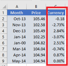
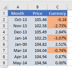
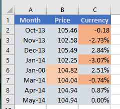
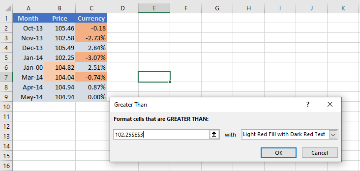
  In this example, we’ll highlight all negative values (price drops) in the “Change” column. So, we select cells C2:C9.

• Go to the Home tab > Styles group, then click Conditional Formatting.
  You’ll see options like Data Bars, Color Scales, and Icon Sets.
• Since we want to highlight numbers less than 0, choose Highlight Cells Rules > Less Than…

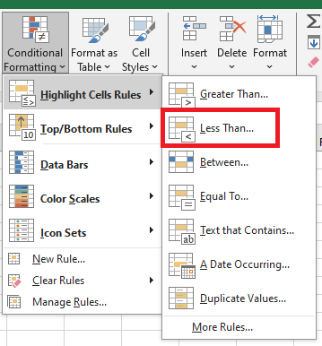
• Other useful rule types include:
  • Format values greater than, less than, or equal to a certain number
  • Highlight cells containing specific text or characters
  • Highlight duplicates
  • Format specific dates
• In the dialog box that appears, enter the value 0 under Format cells that are LESS THAN. Excel will instantly highlight all cells in the selected range that meet the condition.

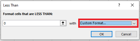
• Select the desired format from the dropdown, or click Custom Format…
• In the Format Cells window, use the Font, Border, and Fill tabs to define your style.
  You’ll see a live preview.
• Click OK to apply the rule.

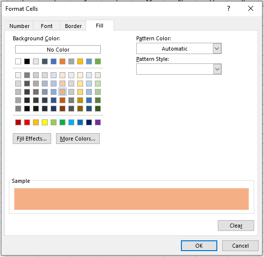
Tip: To access more fill or font colors, click More Colors… in the Font or Fill tab. To apply a gradient background, use Fill Effects.

Create a Custom Rule from Scratch

If none of the default rules meet your needs, you can create one from scratch:

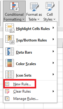
• Select the cells, click Conditional Formatting > New Rule.

• In the dialog, choose a rule type. For example, “Format only cells that contain” and select between 103 and 104.9.

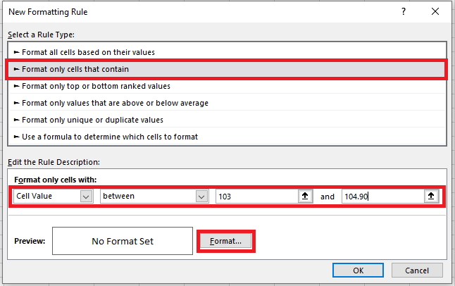
• Click Format… to choose styles.
• Click OK twice to apply the rule.

Format Based on Another Cell’s Value

Instead of typing a number in the rule, you can base it on another cell’s value. This is dynamic—when the referenced cell changes, the formatting updates automatically.

Example: In the “Oil Prices” table, highlight all prices in column B that are higher than the price in B5 (February).

Use Conditional Formatting > Highlight Cell Rules > Greater Than…, and select B5 instead of entering a number.

This is a simple example. For more complex scenarios, use formulas—explained in the article: How to change a cell color based on another cell’s value.

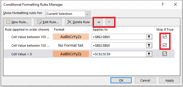
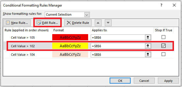
Apply Multiple Conditional Formatting Rules

You’re not limited to one rule per cell. You can apply several rules to the same cell/table.

Example: In a weather table, shade temperatures:

• Above 102 in yellow
• Above 104 in orange
• Above 105 in red

Steps:

• Create the rules with Highlight Cell Rules > Greater Than…
• Go to Conditional Formatting > Manage Rules
• Use the arrows to set rule order (priority)
• Check Stop If True for the first two rules to prevent overlap

Use « Stop If True » in Rules

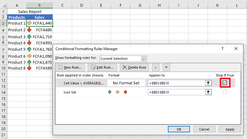
We used Stop If True above to stop lower-priority rules once a condition is met.

Two useful examples:

Example 1: Show Only Down Arrows in Icon Set

Suppose you apply an icon set (arrows) to your sales report:

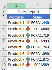
You want to keep only red down arrows for underperformers.

Steps:

• Create a rule: New Rule > Format only cells that contain
• Use the formula =A2>AVERAGE($A$2:$A$10) (adjust cell refs)

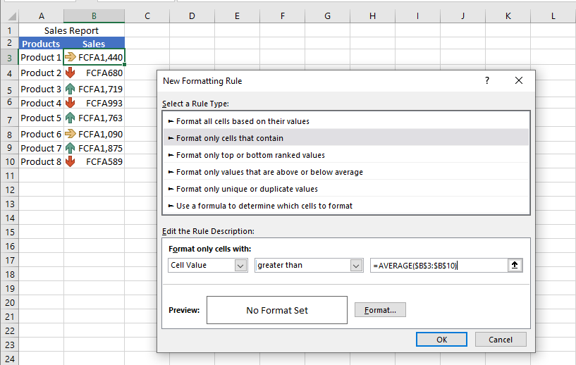
• Leave formatting blank.
• Go to Manage Rules, and check Stop If True for the new rule.

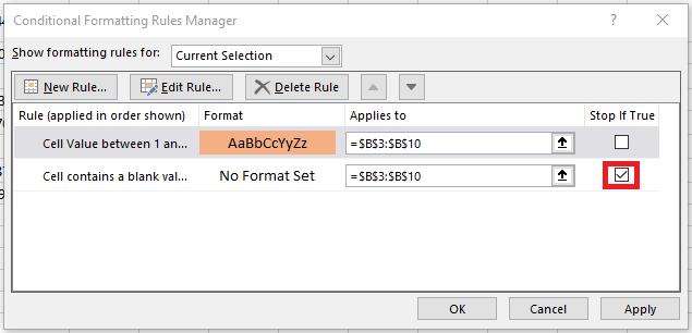
Example 2: Exclude Blank Cells from Formatting

You create a rule like “Between $0 and $1,000”, but empty cells also get highlighted.

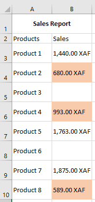
Fix it by:

• Creating a new rule: Format only cells that contain
• Choose Blanks

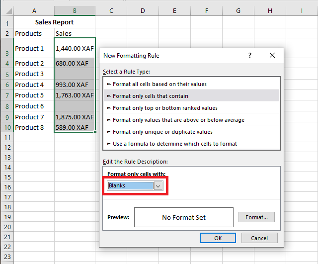
• Leave formatting blank, click OK
• In Manage Rules, check Stop If True next to the blank rule

Edit Conditional Formatting Rules

To edit an existing rule:

• Select a cell with the rule
• Click Conditional Formatting > Manage Rules
• In the Rules Manager, select the rule and click Edit Rule

• Make changes and click OK

If you don’t see your rule, select This Worksheet in the dropdown at the top of the Rules Manager.

Copy Conditional Formatting

To apply a rule from one range to another:

• Click a cell with the rule
• Click Home > Format Painter (mouse turns into a brush)

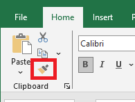
• Drag across the new range to apply formatting
• Press Esc to exit the tool

Note: If your rule uses formulas, you may need to adjust cell references afterward.

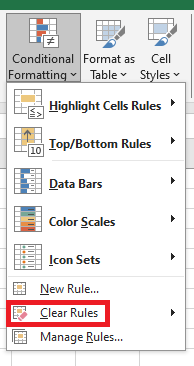
Delete Conditional Formatting Rules

Easiest part

To delete a rule:

• Open Conditional Formatting > Manage Rules, select the rule, click Delete Rule
• Or select the range, go to Conditional Formatting > Clear Rules, and pick from the options

You now have a solid understanding of basic Excel conditional formatting. In the next article, we’ll cover advanced features to push conditional formatting even further in your spreadsheets.

Worksheets with a large amount of data can often appear cluttered and difficult to understand. Fortunately, Microsoft Excel provides a powerful Subtotal feature that allows you to quickly summarize different groups of data and create an outline for your worksheets.

What Is a Subtotal in Excel?

Generally speaking, a subtotal is the sum of a set of numbers, which is then added to one or more other sets to form a grand total. In Microsoft Excel, the Subtotal feature is not limited to summing subsets of values in a dataset. It lets you group and summarize your data using SUM, COUNT, AVERAGE, MIN, MAX, and other functions.

In addition, it creates a hierarchy of groups, known as an outline, which enables you to show or hide details for each subtotal, or just view a summary of the subtotals and grand totals.

For example, here’s what Excel subtotals might look like:

To quickly insert subtotals in Excel, follow these steps:

Organize the Source Data
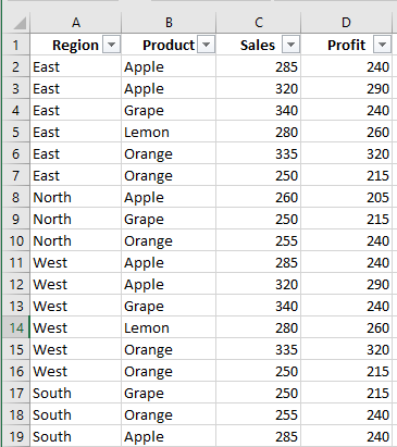
The Excel Subtotal feature requires the source data to be properly sorted and free of blank rows.
So before adding subtotals, make sure to sort the column by which you want to group your data. The easiest way is to click the Filter button on the Data tab, then click the filter arrow and choose Sort A to Z or Sort Z to A: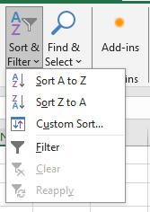

Add Subtotals
Select any cell in your dataset, go to the Data tab > Outline group, then click Subtotal.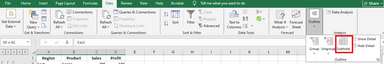

Tip: To subtotal only part of your data, select the desired range before clicking the Subtotal button.

Define Subtotal Options
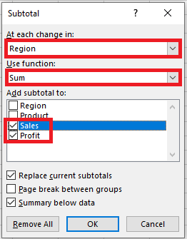
In the Subtotal dialog box, specify the three main elements — which column to group by, which summary function to use, and which columns to subtotal:

• In the At each change in box, select the column that contains the group data.
• In the Use function box, select one of the following:
  • Sum – Adds the numbers
  • Count – Counts non-empty cells (uses COUNTA)
  • Average – Calculates the mean
  • Max – Returns the largest value
  • Min – Returns the smallest value
  • Product – Multiplies the numbers
  • Count Numbers – Counts only numeric cells (uses COUNT)
  • StDev – Estimates standard deviation (sample)
  • StDevP – Standard deviation (population)
  • Var – Estimates variance (sample)
  • VarP – Variance (population)
• Under Add subtotal to, check the columns you want to subtotal.

In this example, we group by the Region column and use the SUM function to total the Sales and Profit columns:

You can also choose:

• Page break between groups – Inserts a page break after each subtotal.
• Summary below data – Uncheck to show the summary row above the data.
• Replace current subtotals – Leave checked to overwrite existing ones.

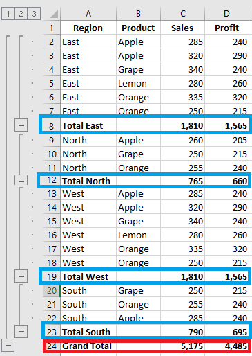
Click OK. Subtotals will appear below each group and a grand total at the bottom.

Once inserted, subtotals are recalculated automatically when source data changes.

Tip: If subtotals are not updating, check File > Options > Formulas > Workbook Calculation and make sure it’s set to Automatic.

Things to Know About Excel Subtotals

The Excel Subtotal feature is powerful and flexible, but also has specific behaviors. Here’s what you need to know:

Only Visible Rows Are Subtotaled
Excel Subtotal only calculates visible cells and ignores filtered-out rows. However, it does include manually hidden rows (e.g., hidden via Home > Format > Hide & Unhide, or right-click > Hide).

It uses the SUBTOTAL function, which includes a function number as its first argument. There are two sets:

• 1–11: Ignores filtered-out cells but includes manually hidden rows.
• 101–111: Ignores both filtered and manually hidden rows.

By default, Excel uses 1–11. For example, using SUM, it will insert:
=SUBTOTAL(9, C2:C7), where 9 means SUM.

To ignore manually hidden rows, change the formula to:
=SUBTOTAL(109, C2:C7), where 109 means SUM (ignoring all hidden rows).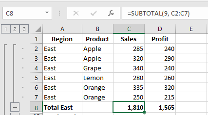

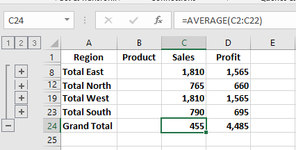
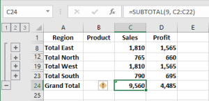
Grand Totals Are Based on Original Data
Grand totals are calculated from raw data, not from subtotal values.

For example, if you use AVERAGE, Excel calculates the grand average from all values in C2:C19, not the subtotal rows.

Subtotals Aren’t Available in Excel Tables
If the Subtotal button is grayed out, you’re likely working with an Excel Table. Subtotals don’t work with tables — convert it to a normal range first.

Adding Multiple (Nested) Subtotals

Let’s now add nested subtotals — for instance, grouping first by Region, then by Item.

Sort Data by Multiple Columns
Go to Data > Sort, and add multiple sort levels (e.g., by Region, then Item).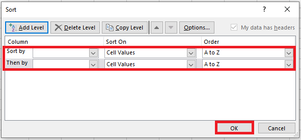

Insert First-Level Subtotals
Select a cell and add the outer subtotal (e.g., by Region as done before).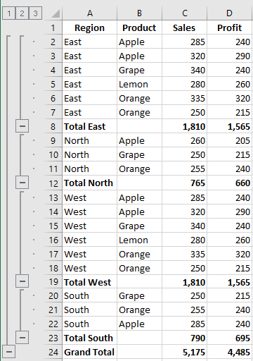

Add Nested Subtotals
Click Data > Subtotal again:

• In At each change in, select the second column (e.g., Item)
• Select a function (e.g., SUM)
• Choose the same or different subtotal columns
• Important: Uncheck Replace current subtotals

Repeat to add more nested subtotals.

Add Different Subtotals for the Same Column

You can apply more than one function to the same column. For example, in addition to the SUM, add AVERAGE for Sales and Profit:

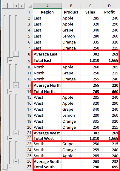
Just follow the steps for adding multiple subtotals and uncheck Replace current subtotals each time.

How to Use Excel Subtotals Effectively

Show or Hide Subtotal Details

Click the outline symbols in the upper-left corner:

• 1 shows only grand totals
• Highest number shows all details
• Intermediate numbers show partial groupings

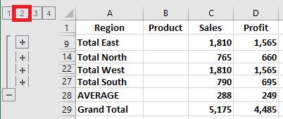
E.g., click 2 to show grouping by Region:

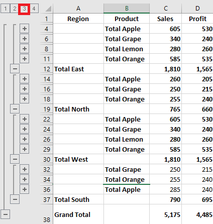
Click 3 to show nested subtotals by Item:

To expand/collapse individual groups, click + / – or use Show/Hide Detail on the Data tab:

Copy Only Subtotal Rows

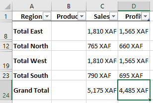
To copy just the visible subtotal rows (not all rows):

• Collapse the outline to display only subtotals
• Select any subtotal cell and press Ctrl + A

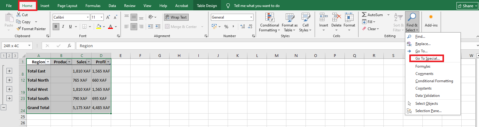
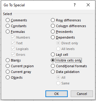
• Go to Home > Find & Select > Go To Special
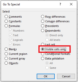
• In the dialog, choose Visible cells only

• Press Ctrl + C to copy, then Ctrl + V to paste elsewhere

This will paste only the subtotal values, not the formulas.

Tip: Use the same method to format all subtotal rows at once.

Modify Existing Subtotals

To quickly change existing subtotals:

• Select a subtotal cell
• Go to Data > Subtotal
• Change the grouping column, summary function, or subtotal columns
• Ensure Replace current subtotals is checked
• Click OK

Note: If multiple subtotals exist for the same data, you must first remove all subtotals and recreate them.

How to Remove Subtotals in Excel

To remove all subtotals:

• Select any cell in the subtotal range
• Go to Data > Outline > Subtotal
• In the dialog box, click Remove All

Besides Excel’s built-in Subtotal tool, there’s also a manual way to add subtotals — by using the SUBTOTAL() function directly. This method offers even more flexibility, and we’ll show you some helpful tricks in the next tutorial

Worksheets containing a lot of complex and detailed information can be difficult to read and analyze. Fortunately, Microsoft Excel provides a simple way to organize data into groups, allowing you to collapse and expand rows with similar content to create more compact and understandable views.

How to Group Rows

Grouping in Excel works best with well-structured worksheets that have column headers, no empty rows or columns, and a summary (subtotal) row for each subset of rows. Once your data is properly organized, use one of the following methods to group it.

Automatically Grouping Rows

If your dataset contains only one level of information, the quickest way is to let Excel group the rows for you. Here’s how:

• Select any cell in one of the rows you want to group.
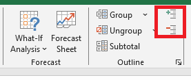
• Go to the Data tab, in the Outline group, click the arrow under Group, and select Auto Outline.

Here is an example of the type of rows Excel can group:

As shown in the screenshot below, the rows are neatly grouped, and outline bars representing different organization levels are added to the left of column A.

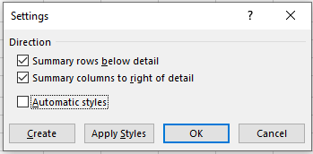
Note: If your summary rows are located above the group of detail rows, go to the Data tab > Outline group, click the Outline Settings dialog launcher, and uncheck Summary rows below detail.

Once the outline is created, you can quickly collapse or expand the details of any group by clicking the minus or plus sign of that group. You can also collapse or expand all rows at a certain level by clicking the level buttons in the upper-left corner of the worksheet.

Manually Grouping Rows

If your worksheet contains at least two levels of information, Excel’s Auto Outline may not group your data correctly. In that case, you can manually group rows by doing the following.

Note: When manually outlining, make sure your dataset does not contain any hidden rows, or your data may be grouped incorrectly.

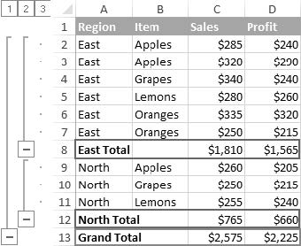
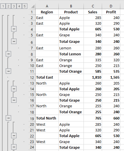
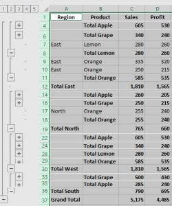
Create Outer Groups (Level 1)
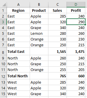
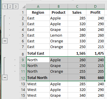
Select one of the largest subsets of data, including all intermediate summary rows and their detail rows. In the example below, to group all data under row 9 (« East Total »), we select rows 2 to 8.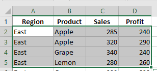

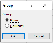
On the Data tab, in the Outline group, click the Group button, select Rows, then click OK.

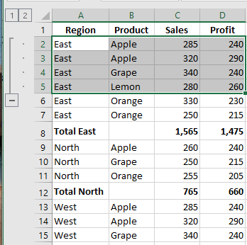
Do the same to create as many outer groups as needed. In this example, we create another outer group for the North region by selecting rows 9 to 12 and clicking Data > Group > Rows:

Tip: To create a new group faster, press Shift + Alt + Right Arrow instead of clicking the Group button on the ribbon.

Create Nested Groups (Level 2)
To create an inner group, select all the detail rows above the related summary row, then click the Group button. For example, to group “Apples” in the East region, select rows 2 and 3 and press Group. Then group “Oranges” by selecting rows 5 to 7. Do the same for the North region: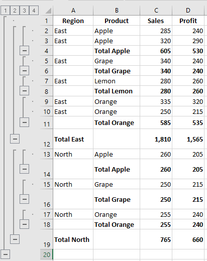

Add More Grouping Levels If Needed
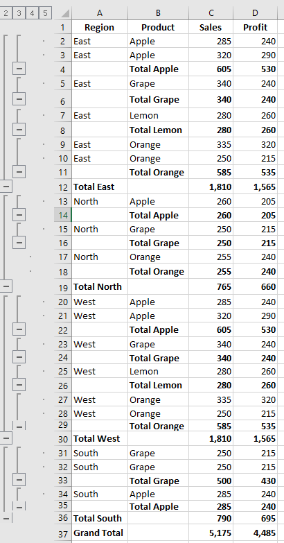
Datasets are rarely final. If you add more data, you may want to insert more outline levels. For instance, after inserting a Grand Total row, select all rows except the Grand Total row (rows 2 to 17), and then click Data > Group > Rows. Now your data has 4 levels:

• Level 1: Grand Total
• Level 2: Region totals
• Level 3: Item subtotals
• Level 4: Detail rows

Now that we’ve outlined the rows, let’s see how this helps with data visualization.

How to Collapse Rows

One of the most useful features of Excel grouping is the ability to hide or show detail rows for a specific group, or collapse/expand the entire outline to a particular level with a single mouse click.

Collapse Rows Within a Group

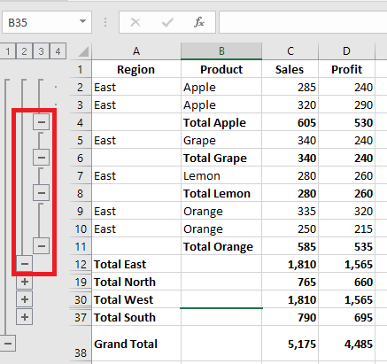
To collapse the rows of a particular group, simply click the minus sign at the bottom of the group’s outline bar. For example, to hide all detail rows for the East region and show only the « East Total » row:

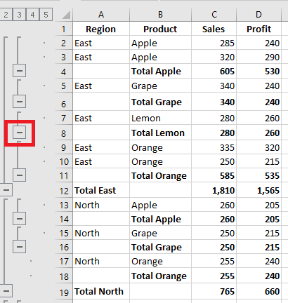
Another way is to select any cell in the group and click Hide Detail on the Data tab in the Outline group:

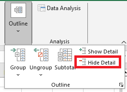
In either case, the group will collapse to just the summary row, and all detail rows will be hidden.

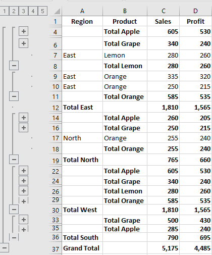
Collapse or Expand the Entire Outline at a Specific Level

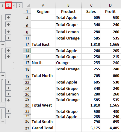
To collapse or expand all groups to a specific level, click the corresponding level number in the upper-left corner of your worksheet. Level 1 shows the least data, while higher numbers expand more rows.

In our dataset with 4 outline levels:

• Level 1: Shows only the Grand Total (row 18)
• Level 2: Grand Total + Regional Totals (rows 9, 17, 18)
• Level 3: Adds Item Subtotals (rows 4, 8, 13, 16)
• Level 4: Shows all detail rows

The screenshot below shows the outline collapsed to level 3:

How to Expand Rows in Excel

To expand a specific group, click any cell in the summary row and then click Show Detail on the Data tab in the Outline group:

Or click the plus sign for the collapsed group you want to expand:

How to Remove the Outline

If you want to remove all grouped rows at once, clear the outline. If you want to remove only specific groups (like nested ones), ungroup the selected rows.

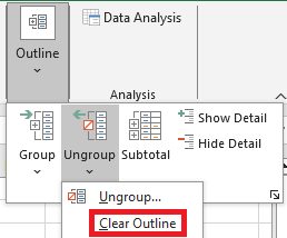
To remove the entire outline:

• Go to the Data tab > Outline group
• Click the arrow under Ungroup, then click Clear Outline

Notes:

• Removing an outline does not delete any data.
• If you clear an outline with collapsed rows, those rows may remain hidden.
• Once the outline is removed, you cannot undo it with Undo (Ctrl + Z). You must recreate the outline from scratch.

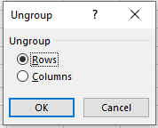
How to Ungroup Specific Rows

To remove grouping from certain rows without deleting the entire outline:

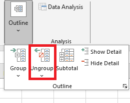
• Select the rows you want to ungroup.
• Go to Data > Outline, click Ungroup or press Shift + Alt + Left Arrow (Excel’s Ungroup shortcut).
• In the Ungroup dialog box, select Rows and click OK.

For example, here’s how to ungroup two nested groups (Apples Subtotal and Oranges Subtotal) while keeping the outer « East Total » group:

Note: You cannot ungroup non-adjacent row groups at once. Repeat the steps for each group individually.

How to Automatically Calculate Group Subtotals

In the above examples, we inserted our own subtotal rows with SUM formulas. To have Excel calculate subtotals automatically, use the Subtotal command with a summary function such as SUM, COUNT, AVERAGE, MIN, MAX, etc.

The Subtotal command will insert summary rows and create an outline with collapsible/expandable rows — two tasks in one!

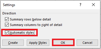
Applying Excel’s Default Styles to Summary Rows

Microsoft Excel provides predefined styles for two levels of summary rows: RowLevel_1 (bold) and RowLevel_2 (italic). You can apply these styles either before or after grouping the rows.

To automatically apply styles to a new outline:

• Go to Data > Outline
• Click the Outline Settings dialog launcher
• Check the Automatic Styles box and click OK

To apply styles to an existing outline, check the same box and click Apply Styles instead of OK.

Here’s what an outlined sheet looks like with default summary row styles:

How to Select and Copy Only Visible Rows

After collapsing unnecessary rows, you may want to copy only the visible (relevant) data. However, selecting rows the usual way with the mouse also selects hidden rows.

To select only visible rows:

• Select the visible rows using the mouse (e.g., only summary rows).

• Go to Home > Editing > Find & Select > Go To Special
  Or press Ctrl + G, then click Special…
• In the Go To Special dialog box, select Visible cells only and click OK.

Only visible rows are now selected (adjacent to hidden ones marked with white borders):

Now press Ctrl + C to copy and Ctrl + V to paste wherever you want.

How to Show or Hide Outline Symbols

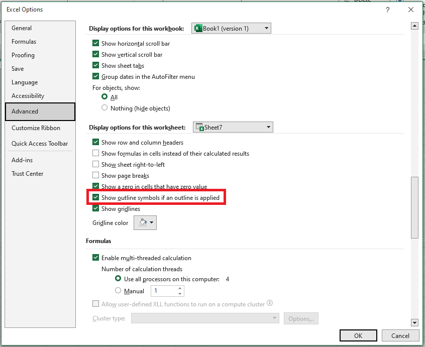
To toggle the display of outline symbols and level numbers, use the shortcut Ctrl + 8. Press once to hide the symbols, press again to show them.

If you do not see the plus/minus symbols or level numbers, check this setting:

• Go to File > Options > Advanced
• Scroll to Display options for this worksheet
• Select your worksheet and ensure Show outline symbols if an outline is applied is checked.

This is how you group rows in Excel to collapse or expand sections of your dataset. Likewise, you can group columns in your worksheets.