Votre panier est actuellement vide !
Étiquette : practical-excel
What Is a Chart in Excel
A chart is a visual representation of numerical values. Charts are an integral part of spreadsheets. The charts generated by early spreadsheet programs were fairly basic, but they have improved significantly over the years. Excel provides you with the tools to create a wide variety of highly customizable, professional-quality charts.
Displaying data in a well-designed chart can make your numbers much easier to understand. Because a chart presents a visual image, charts are especially useful for summarizing a series of numbers and their relationships. Creating a chart can often help you spot trends and patterns that might otherwise go unnoticed.
The following figure shows a worksheet that contains a simple column chart representing a company’s monthly sales volume.
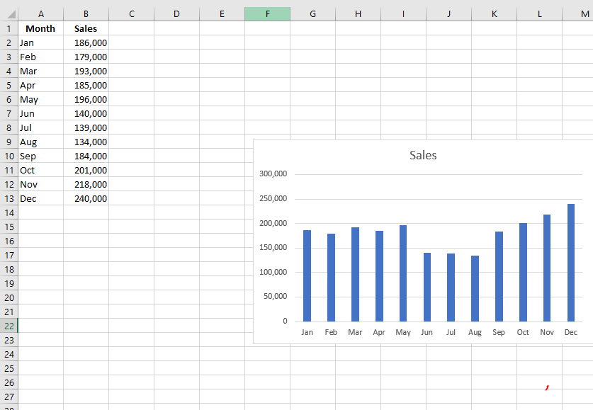
A quick glance at the chart clearly reveals that sales dropped during the summer months (June through August), but steadily increased over the last four months of the year. Of course, you could reach the same conclusion simply by studying the numbers. However, visualizing the data through a chart conveys the point much more quickly.
A simple column chart represents monthly sales volume.
Formatting Text Using the CONCATENATE Function in Excel
In your Excel workbooks, data is not always structured the way you need. Often, you may want to split the content of one cell into multiple cells—or do the opposite: combine data from two or more columns into one.
Common examples that require concatenation in Excel include combining names and address parts, merging text with formula-based values, and formatting dates and times as desired, to name just a few.The Excel CONCATENATE function joins up to 30 values together and returns the result as a single text string. Its syntax is:
=CONCATENATE(text1, text2, [text3], ...)
- text1 – The first text value to join.
- text2 – The second text value to join.
- text3 – (optional) The third text value to join.
The values can be cell references or hardcoded text strings. Only the first argument is required, and the values are concatenated in the order they appear.
For example, to concatenate the values in cells A1 and B1, separated by a space, you can use CONCATENATE as follows:
=CONCATENATE(A1, " ", B1)
The result of this formula is the same as using the ampersand (
&) operator manually like this:= A1 & " " & B1 // manual concatenation
The ampersand character (
&) is an alternative to the CONCATENATE function. The result is the same, but the ampersand is more flexible and creates shorter (and arguably more readable) formulas.Join Text Strings
One of the most basic text manipulation tasks you can perform is joining text strings. In the example shown in the figure below, you create a full name column by joining first and last names.
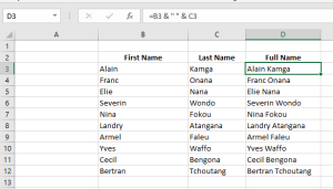
This example uses the ampersand operator (
&). The ampersand tells Excel to concatenate the values together. As shown in the figure, you can combine cell values with any custom text. In this case, values in cells B3 and C3 are joined with a space between them (entered as" "in quotes).Note:
Excel also offers a CONCATENATE function that joins values without using the ampersand. In this example, you could also write:=CONCATENATE(B3, " ", C3)
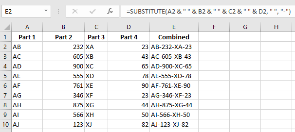
Use the SUBSTITUTE Function to Combine and Separate ColumnsThe ampersand (
&) operator is commonly used to combine multiple columns into a single one.
To include a separator between the parts (instead of just blank spaces), you can define the separator once and use the SUBSTITUTE function as follows:To combine and separate at the same time:
- Enter any type of data in columns A through D.
- Select cells F2:F10 and enter the following formula:
=SUBSTITUTE(A2 & " " & B2 & " " & C2 & " " & D2, " ", "-")- Press Ctrl + Enter.
Formatting Text Using the UPPER, LOWER, and PROPER Functions in Excel
Use the UPPER Function to Convert Text from Lowercase to Uppercase
The UPPER function is used to convert a text string to all uppercase letters. Its syntax is:
UPPER(text)- text: The text you want to convert to uppercase. This can be a text string or a cell reference.
To convert text to uppercase:
- In cells A2:A8, enter any text in lowercase.
- Select cells B2:B8 and enter the following formula:
=UPPER(A2) - Press Ctrl + Enter.

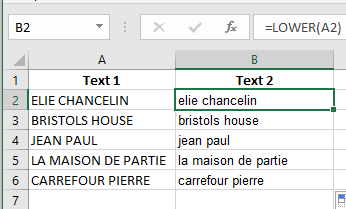
Use the LOWER Function to Convert Text from Uppercase to Lowercase
To convert all letters in a text string to lowercase, use the LOWER function. Its syntax is:
LOWER(text)- text: The text you want to convert to all lowercase. It can be a text string or a reference.
To convert text to lowercase:
- In cells A2:A8, enter any text in uppercase.
- Select cells B2:B8 and enter the following formula:
=LOWER(A2) - Press Ctrl + Enter.
Use the PROPER Function to Capitalize the First Letter of Each Word
To convert the first letter of each word to uppercase and the remaining letters to lowercase, use the PROPER function. This function capitalizes the first letter of a text string and each letter that follows a non-letter character (such as a space). All other letters are converted to lowercase.Syntax:
PROPER(text)- text: Text in quotation marks, a formula that returns text, or a reference to a cell containing the text to be capitalized.
To convert text to title case:
- In cells A2:A6, enter any type of text with different capitalization patterns.
- Select cells B2:B7 and enter:
=PROPER(A2) - Press Ctrl + Enter.

Change Text to Uppercase, Lowercase, or Title Case
Excel provides three helpful functions to convert text to uppercase, lowercase, or title case.
As shown in rows 6, 7, and 8 of the following figure, these functions only need a pointer to the text you want to convert.- The UPPER function converts text to all uppercase.
- The LOWER function converts text to all lowercase.
- The PROPER function converts text to title case (the first letter of each word is capitalized).
What Excel lacks is a built-in function to convert text to sentence case (only the first letter of the first word capitalized). However, you can use the following formula to force sentence case:
=UPPER(LEFT(C4,1))&LOWER(RIGHT(C4,LEN(C4)-1))If you look closely at this formula, you’ll see it consists of two parts joined by an ampersand
&.The first part uses Excel’s LEFT function:
UPPER(LEFT(C4,1))
The LEFT function extracts a specified number of characters from the start of a text string.
It takes two arguments: the text and the number of characters to extract.
In this case, it extracts the first character of cell C4 and converts it to uppercase with the UPPER function.The second part is more complex. It uses the RIGHT function:
LOWER(RIGHT(C4,LEN(C4)-1))
Like LEFT, the RIGHT function takes two arguments: the text and how many characters to extract from the end.
Instead of hardcoding the number, it calculates it by subtracting 1 from the total length of the text using the LEN function.
This is because the first character has already been capitalized by the LEFT/UPPER part.Finally, the RIGHT portion is wrapped in the LOWER function to convert the rest of the text to lowercase.
Putting it all together gives you sentence case:
=UPPER(LEFT(C4,1))&LOWER(RIGHT(C4,LEN(C4)-1))Formatting Text Using the LEFT, RIGHT, and MID Functions in Excel
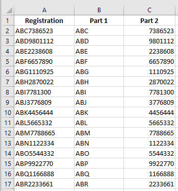
Use the LEFT and RIGHT functions to split a text string of digits
A worksheet contains a list of 10-digit numbers that need to be split into two parts: a three-digit part and a seven-digit part. Use the LEFT and RIGHT functions to do this. The LEFT function returns the first character(s) in a text string, based on the number of characters specified. The RIGHT function returns the last character(s) in a text string based on the number of characters specified.Syntax of the LEFT function:
LEFT(text, [num_chars])The LEFT function has the following arguments:
■ text (Required). The text string that contains the characters you want to extract.
■ num_chars (Optional). Specifies the number of characters to return.- num_chars must be greater than or equal to zero.
- If num_chars is greater than the length of text, the function returns the entire text.
- If omitted, the default value of num_chars is 1.
Syntax of the RIGHT function:
RIGHT(text, [num_chars])The RIGHT function includes the following arguments:
■ text (Required). The text string that contains the characters you want to extract.
■ num_chars (Optional). The number of characters to return.- Must be greater than or equal to zero.
- If it exceeds the length of text, the entire text is returned.
- If omitted, the default is 1.
To split a string of digits:
- In a worksheet, enter a series of 10-character numbers in cells A2:A17. Letters may also be included.
- Select cells B2:B17 and type:
=LEFT(A2,3) - Press Ctrl+Enter.
- Select cells C2:C17 and type:
=RIGHT(A2,7) - Press Ctrl+Enter.
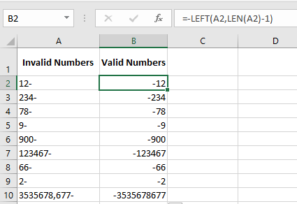
Use the LEFT function to convert invalid numbers into valid ones
In this example, invalid numbers must be corrected. These numbers contain a minus sign at the end.
Excel cannot interpret this correctly, so the minus sign must be moved to the left of the number.
First, use the LEN function to determine the length of each number. Then use LEFT to shift the minus sign.Syntax of the LEN function:
LEN(text)■ text (Required). The text whose length you want to determine. Spaces count as characters.
To cut the last character and display a negative value:
- Enter a series of numbers with a trailing minus sign in cells A2:A10.
- Select B2:B10 and enter:
= -LEFT(A2, LEN(A2)-1) - Press Ctrl+Enter.
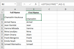
Use the FIND function to split the first name from the last name
This task shows how to separate first and last names. Full names are listed in column A.
We want to extract the first name into column B. The FIND function can locate the space separating the two parts.Syntax:
FIND(find_text, within_text, [start_num])■ find_text: The character or text to locate. You can use wildcards:
?(any single character),*(any sequence). Use~before a wildcard to search for the literal character.
■ within_text: The text where you search.
■ start_num: The position to start the search. Default is 1.Examples:
=FIND("n", "printer")returns 8
=FIND("form", "platform")returns 6To extract the first name:
- Enter full names in A2:A10.
- Select B2:B11 and type:
=LEFT(A2, FIND(" ", A2)-1) - Press Ctrl+Enter
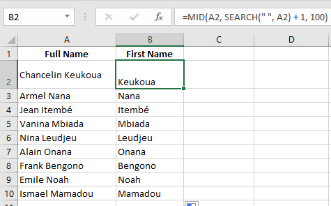
Use the MID function to extract the last name
Full names are listed in column A. We want to extract the last name into column B.
Use FIND to identify the space, then use MID to return characters starting just after it.Syntax:
MID(text, start_num, num_chars)■ text (Required). The string containing the characters to extract.
■ start_num (Required). Position of the first character to extract.- If start_num > length of text, MID returns an empty string.
- If start_num + num_chars > length, MID returns the rest of the string.
- If start_num < 1, MID returns #VALUE!
■ num_chars (Required). Number of characters to extract. - If negative, returns #VALUE!
To extract the last name:
- Enter full names in A2:A10.
- Select B2:B11 and type:
=MID(A2, FIND(" ", A2)+1, 100) - Press Ctrl+Enter
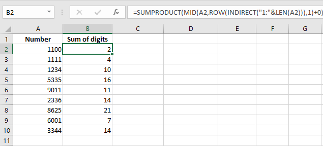
Use the MID function to sum digits in a number
The worksheet contains 4-digit numbers in column A.
We want to sum the digits of each number. Use MID to extract each digit and add them.To calculate the digit sum:
- Enter 4-digit numbers in A2:A10.
- Select B2:B10 and enter:
=MID(A2,1,1)+MID(A2,2,1)+MID(A2,3,1)+MID(A2,4,1) - Press Ctrl+Enter
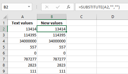
Use the SUBSTITUTE function to replace characters
Column A contains values formatted as text.
Use the SUBSTITUTE function to replace specific characters.Syntax:
SUBSTITUTE(text, old_text, new_text, [instance_num])■ text (Required). The string or cell reference.
■ old_text (Required). The text to be replaced.
■ new_text (Required). The replacement text.
■ instance_num (Optional). Specifies which occurrence to replace.
If omitted, all instances of old_text are replaced.To make Excel recognize text as numbers:
- Format column A as text.
- Enter numbers (as text) in A2:A10.
- In B2:B10, enter:
=SUBSTITUTE("'" , " ")(This example seems incorrect — see note) - Press Ctrl+Enter.
- In A12:
=SUM(A2:A10) - In B12:
=SUM(B2:B10)
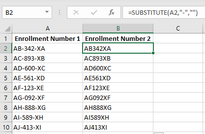
Use SUBSTITUTE to replace parts of a cell
To replace a character:- Select B2:B9 and type:
=SUBSTITUTE(A2, "-", "", 1) - Press Ctrl+Enter
Note: To replace the second occurrence, use:
=SUBSTITUTE(A2, "-", "", 2)
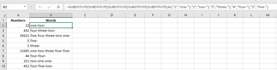
Use SUBSTITUTE to convert digits into words
The worksheet contains numbers 1 to 5 in column A.
Use nested SUBSTITUTE functions to convert them into words.To convert digits to words:
- Enter numbers 1–5 in column A.
- In B2:B10, enter:
=SUBSTITUTE(SUBSTITUTE(SUBSTITUTE(SUBSTITUTE(SUBSTITUTE(A2,1,"one-"),2,"two-"),3,"three-"),4,"four-"),5,"five-")
Use SUBSTITUTE to remove carriage return characters
To wrap text in a cell: use the Wrap Text option or press Alt+Enter to insert line breaks.
To remove line breaks, use SUBSTITUTE with the CHAR function.
The ASCII code for line break is 10.To remove line breaks:
- Enter multi-line text in cell A2.
- In B2, type:
=SUBSTITUTE(A2, CHAR(10), " ") - Press Ctrl+Enter

Performing Statistical Operations Using the COUNTIF Function in Excel
The COUNTIF function is used to count the number of cells in a specified range that meet a certain condition or criterion.
For example, you can write a COUNTIF formula to find how many cells in your worksheet contain values greater or less than a specified number.
Another common use of COUNTIF in Excel is to count cells containing a specific word or starting with one or more specific letters.Syntax:
=COUNTIF(range, criteria)As you can see, the function takes only two required arguments:
■ range – Defines one or more cells to count. You enter the range just like any other range in Excel (e.g., A1:A20).
■ criteria – Defines the condition that tells the function which cells to count. It can be a number, text string, cell reference, or expression.Use the COUNTIF Function to Count Phases Costing More Than 1,000
In this example, different project phases are listed in a worksheet. To determine how many of them cost more than 1,000, use the COUNTIF function.
This function counts how many cells in a range meet the specified condition.To count the specified phases:
- In cells A2:A11, enter the names of the various project phases.
- In cells B2:B11, enter the cost of each phase.
- In cell D1, enter
1000as the given threshold. - Select cell D2 and type the following formula:
=COUNTIF(B2:B11, ">" & D1) - Press Enter.
NOTE:
If you don’t want to link the criteria to a cell reference, use the formula:
=COUNTIF(B2:B11, ">1000")Use the COUNTIF Function to Calculate Attendance
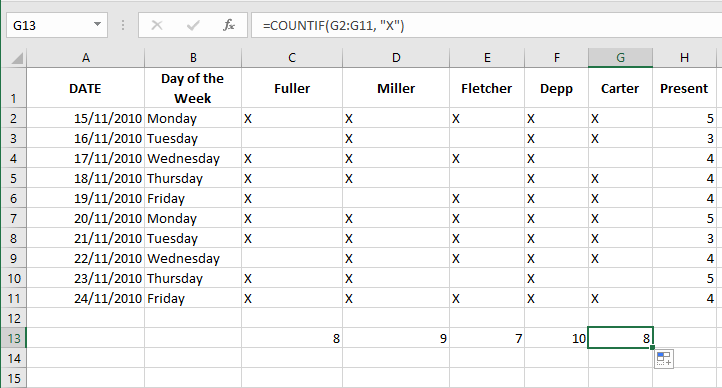
In this task, you want to generate an attendance list and determine how many people were present each day.
Create a table similar to the one shown in Figure 6–7.
Column A contains dates, and column B uses a custom format to display the weekday.
In columns C to G, the letter « X » is entered for each person present.To calculate daily attendance:
- Select cells H2:H11 and type the formula:
=COUNTIF(C2:G2, "X")
This counts attendance per day. - Press Ctrl+Enter.
- To calculate total attendance for each employee, select cells C13:G13 and type:
=COUNTIF(C2:C11, "X"),=COUNTIF(D2:D11, "X"), etc. (or use relative references like=COUNTIF(G2:G11, "X")) - Press Ctrl+Enter.
Performing Logical Operations Using the AVERAGEIF Function in Excel
The AVERAGEIF function in Excel calculates the average of cells that meet a specific criterion.
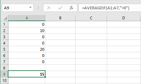
It returns the arithmetic mean of values that match a condition.The formula below (with two arguments) calculates the average of all values in range A1:A7 that are greater than 0:
=AVERAGEIF(A1:A7, ">0")
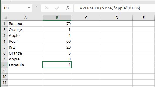
The formula below (with three arguments; the last one is the range to average) calculates the average of values in B1:B6 where the corresponding A1:A6 cells equal « Apple »:
=AVERAGEIF(A1:A7, "Apple", B1:B6)
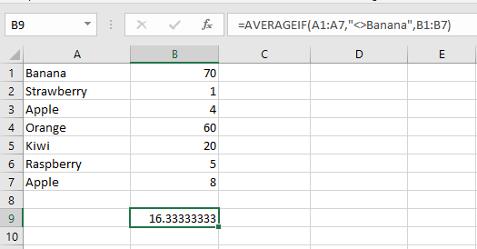
The formula below calculates the average of values in B1:B7 where the corresponding cells in A1:A7 are not equal to « Banana »:
=AVERAGEIF(A1:A7, "<>Banana", B1:B7)
The formula below averages the values in B1:B7 where the corresponding A1:A7 cells contain any characters followed by « berry ».
Use an asterisk*as a wildcard to represent any sequence of characters:
=AVERAGEIF(A1:A7, "*berry", B1:B7)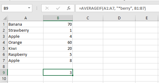
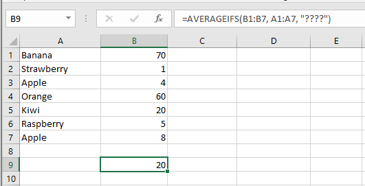
The formula below averages values in B1:B7 where the corresponding A1:A7 cells contain exactly four characters.
Use a question mark?as a wildcard for a single character:
=AVERAGEIF(A1:A7, "????", B1:B7)
The AVERAGEIFS function (note the final S) calculates the average based on multiple criteria.
This formula calculates the average of values in A1:A7 that are ≥ 500 and ≤ 1000:
=AVERAGEIFS(A1:A7, A1:A7, ">=500", A1:A7, "<=1000")Note: The first argument is the range to average, followed by one or more pairs of range/criteria.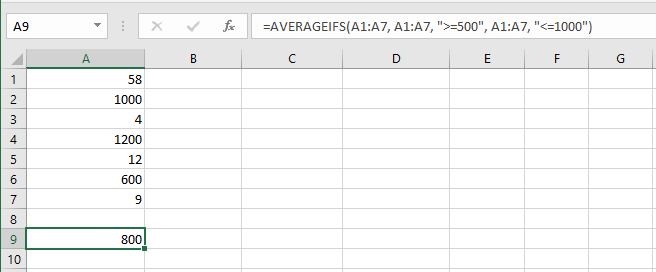
7. This formula averages the values in C1:C7 where the corresponding cells in A1:A7 equal « Apple » and the corresponding cells in B1:B7 equal « Red »:
=AVERAGEIFS(C1:C7, A1:A7, "Apple", B1:B7, "Red")Note: Again, the first argument is the range to average, followed by multiple range/criteria pairs.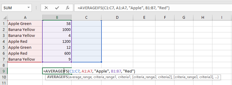
Performing Logical Operations Using the SUMIF Function in Excel
SUMIF is used to add values based on a single condition. With this function, you can calculate the total of numbers that meet a specific criterion within a range. It belongs to the Math & Trigonometry category and is commonly used to extract the total of specific numbers from large datasets.
Syntax:
=SUMIF(range, criteria, [sum_range])■ range: The range of cells to evaluate with the condition
■ criteria: The condition to be met
■ sum_range: The actual range to sum if the condition is metUse the SUMIF Function to Determine a Team’s Sales
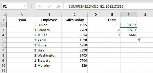
In this example, you want to total the sales of different teams.
SUMIF allows you to sum values from a range based on a given criterion.To sum specified data:
- In cells A2:A10, enter team numbers from 1 to 3.
- List the team members in cells B2:B10.
- In cells C2:C10, enter each employee’s daily sales.
- In cells E2:E4, list the numbers 1, 2, and 3 for each team.
- Select cells F2:F4 and enter the following formula:
=SUMIF($A$2:$A$10, E2, $C$2:$C$10) - Press Ctrl+Enter.
Use the SUMIF Function to Total Costs Greater Than 1,000
This trick helps determine the total cost of phases with costs greater than $1,000.
To add only those cells, use the SUMIF function with a greater-than condition.To sum specified costs:
- In cells A2:A11, list the different phases.
- Enter the cost of each phase in cells B2:B11.
- In cell D1, enter
1000as the threshold. - In cell D2, enter the formula:
=SUMIF(B2:B11, ">" & D1) - Press Enter.
NOTE:
If the criteria are not linked to a cell reference, use the formula:
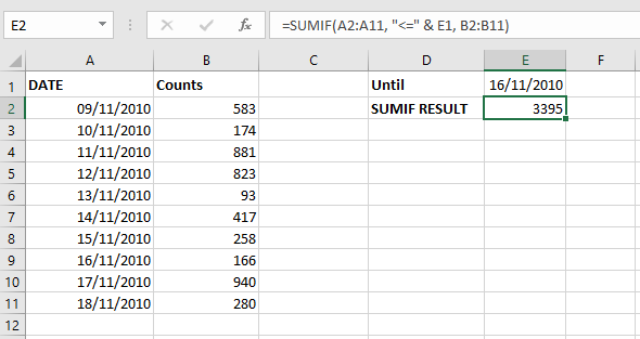
=SUMIF(B2:B11, ">1000")Use the SUMIF Function to Sum Costs Up to a Specific Date
To sum all costs before or on a specific date, use SUMIF with a date condition.
To sum costs up to a given date:
- In cells A2:A11, list the dates from 11/09/10 to 11/18/10.
- In cells B2:B11, enter the corresponding daily costs.
- In cell E1, enter the date
11/16/10. - In cell E2, type the following formula:
=SUMIF(A2:A11, "<=" & E1, B2:B11) - Press Enter.
NOTE:
To verify the calculated result, select cells B2:B9 and observe the total shown in Excel’s status bar.
Performing Logical Operations Using the IF Function in Excel
The IF function performs a logical test and returns one value for a TRUE result and another for a FALSE result.
Syntax:
=IF(condition, value_if_true, value_if_false)Where:
■ condition: A value or logical expression that can be evaluated as TRUE or FALSE.
■ value_if_true (optional): The value to return if the condition is TRUE.
■ value_if_false (optional): The value to return if the condition is FALSE.An IF statement therefore has two possible outcomes: the first result is applied if the condition is met (TRUE), otherwise the second result is applied.
Example:
IF(C2="Yes", 1, 2)means:
If C2 = « Yes », return 1; otherwise return 2.Use the IF Function to Compare Columns and Return a Specific Result
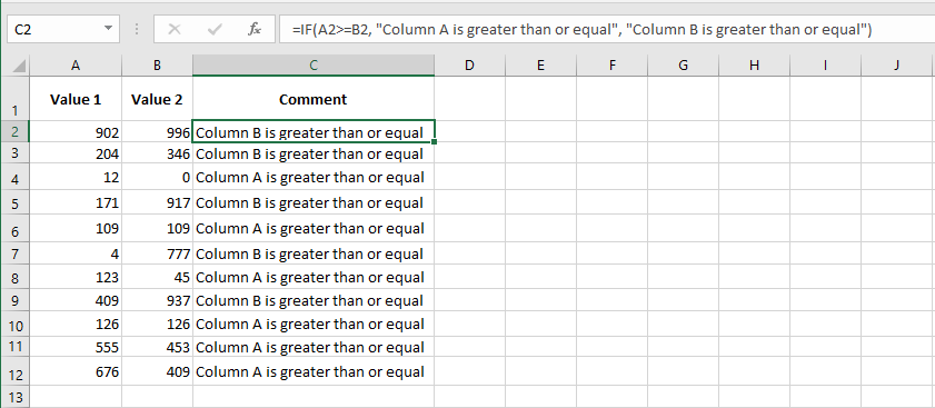
This example compares two columns and displays the result in column C.
To return specific text after comparing values:
- Enter values between 0 and 1,000 in range A2:A12.
- Enter values between 0 and 1,000 in range B2:B12.
- Select cells C2:C12 and type the following formula:
=IF(A2>=B2, "Column A is greater or equal", "Column B is greater or equal") - Press Ctrl+Enter.
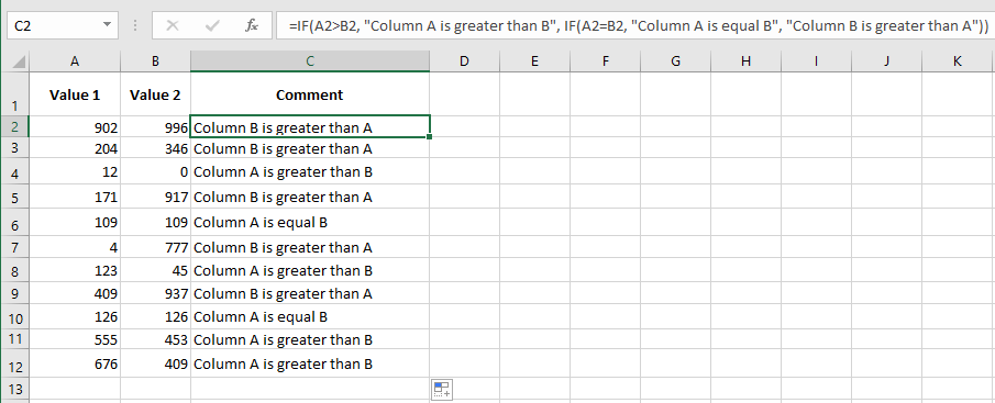
Use the IF Function to Check for Greater, Equal, or Lesser Values
In the previous example, two different messages were returned.
To check for three outcomes— »Column A is greater », « Equal », or « Column A is smaller »—proceed as follows:- Copy the previous example.
- Select cells C2:C12 and type:
=IF(A2>B2, "Column A is greater", IF(A2=B2, "Equal", "Column A is smaller")) - Press Ctrl+Enter.
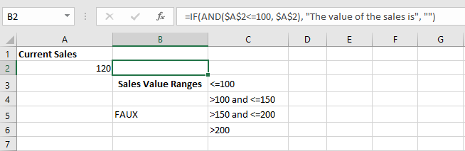
Combine IF with AND to Check Multiple Conditions
In this example, Excel evaluates conditions and returns the result on the same row.
To combine IF and AND:
- Copy the content of cells C2:C5 from the figure into your Excel sheet.
- Format the table as shown.
- In cell A2, enter a sales amount (e.g., 120).
- In cell B2, enter:
=IF(AND($A$2<=100, $A$2), "Sales value is", "") - In cell B3, enter:
=IF(AND($A$2>100, $A$2<=150), "Sales value is", "") - In cell B4, enter:
=IF(AND($A$2>150, $A$2<=200), "Sales value is", "") - In cell B5, enter:
=IF($A$2>200, "Sales value is", "")
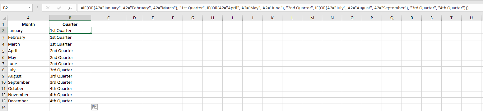
Use the IF Function to Determine the Quarter of the Year
After typing a start value, Excel can auto-fill cells with months.
In a new worksheet, type « January » in A2, then drag down to A13.
To show which months belong to which quarter:- Select cells B2:B13 and enter:
=IF(OR(A2="January", A2="February", A2="March"), "Q1", IF(OR(A2="April", A2="May", A2="June"), "Q2", IF(OR(A2="July", A2="August", A2="September"), "Q3", "Q4"))) - Press Ctrl+Enter.
Use the IF Function Across Worksheets and Workbooks
To use IF in another worksheet or linked workbook, start typing the formula (e.g.
=IF(), then navigate to the other sheet or file, select the cell, and return to finish.For referencing another worksheet:
=IF(Sheet8!A2="January", "Bad", "OK")For referencing another workbook:
=IF('C:\Chancelin\Formulas\Files\[Formulas.xls]Sheet35'!$A$1<>1, "Bad", "OK")NOTE: For this to work, the referenced sheet or file must exist. It can be tested by changing the sheet or file name.Use the IF Function to Calculate with Different Tax Rates
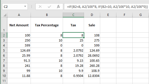
To handle different tax rates in calculations, use nested IF functions.
- In column A, enter item prices.
- In column B, enter tax rates (0, 8, or 10).
- Select cells C2:C10 and type:
=IF(B2=8, A2*8/100, IF(B2=10, A2*10/100, A2*0/100)) - Press Ctrl+Enter.
- In D2:D10, type:
=A2+C2 - Press Ctrl+Enter.
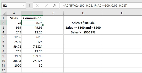
Use the IF Function to Calculate Sales Commissions
A company uses different commission rates:
- Sales < $100 → 3%
- Sales ≥ $100 and < $500 → 5%
- Sales ≥ $500 → 8%
- Enter different sales amounts in column A.
- In cells B2:B12, enter:
=A2*IF(A2>=500, 0.08, IF(A2>=100, 0.05, 0.03)) - Press Ctrl+Enter.
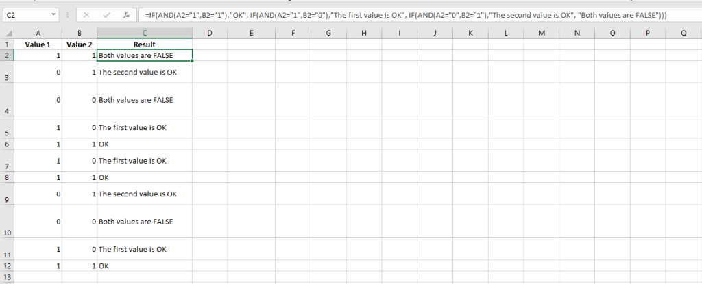
Use the IF Function to Compare Two Cells
This trick compares two cells row by row. Prepare a new sheet with 0s and 1s in columns A and B.
- In cells C2:C11, enter:
=IF(A2&B2="11", "OK", IF(A2&B2="10", "First value OK", IF(A2&B2="01", "Second value OK", "Both values are FALSE"))) - Press Ctrl+Enter.
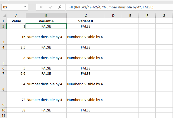
Use the INT Function with IF to Test Integer Divisibility
To check if a number is divisible by 4:
- In B2:B10, type:
=IF(INT(A2/4)=A2/4, "Integer divisible by 4", FALSE) - Press Ctrl+Enter
OR
- In C2:C10, type:
=IF(A2/4-INT(A2/4)=0, "Integer divisible by 4", FALSE) - Press Ctrl+Enter
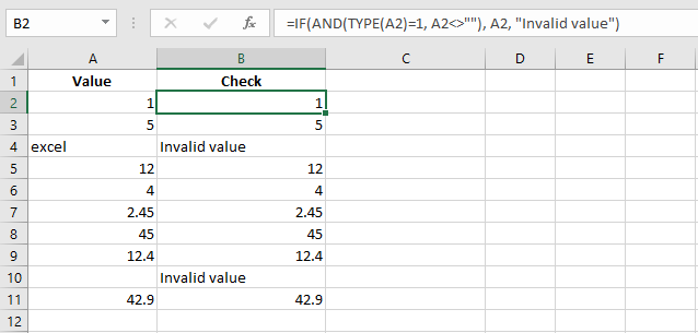
Use TYPE with IF to Check for Invalid Values
Excel may misinterpret imported values. To detect invalid values, combine IF with TYPE.
This example returns « invalid value » in column B if the entry in A is not numeric.- Enter numbers or text in column A.
- In B2:B10, enter:
=IF(AND(TYPE(A2)=1, A2<>""), A2, "invalid value") - Press Ctrl+Enter
Use IF More Than Seven Times in One Cell
Excel’s documentation says you can’t nest IF more than seven times. That’s not true:
- In cell A2, enter
12. - In B2, enter:
=IF(A2=1,A2,IF(A2=2,A2*2,IF(A2=3,A2*3,IF(A2=4,A2*4,IF(A2=5,A2*5,IF(A2=6,A2*6,IF(A2=7,A2*7,""))))))+IF(A2=8,A2*8,IF(A2=9,A2*9,IF(A2=10,A2*10,"")))+IF(A2=11,A2*11,IF(A2=12,A2*12,""))

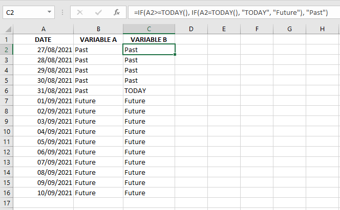
Use the IF Function to Check if a Date is in the Past or Future
To check whether a date is in the past or future, use TODAY() with IF.
Variant A:
- In B2:B16, enter:
=IF(NOT(A2>TODAY()), "Past", "Future") - Press Ctrl+Enter
Variant B:
- In B2:B11, enter:
=IF(A2>=TODAY(), IF(A2=TODAY(), "Today", "Future"), "Past") - Press Ctrl+Enter
Performing Calculations Using the AVERAGE Function in Excel
The AVERAGE function in Excel calculates the average (arithmetic mean) of a group of numbers. The AVERAGE function ignores logical values, empty cells, and text values.
Syntax:
=AVERAGE(number1, [number2], …)Where:
■ number1 (required argument) – The first reference or range of items or cells for which you want to calculate the average.
■ number2… (optional argument) – You can add up to 255 additional items, cell references, or ranges in which to calculate the average.You can use ranges or cell references instead of explicit values. The AVERAGE function can handle up to 255 arguments, each of which may be a value, a cell reference, or a range.
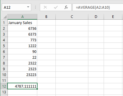
This example calculates the average of January sales using the AVERAGE function, which returns the arithmetic mean of the arguments.
=AVERAGE(number1, number2, …)NOTE:To determine the last filled column in a worksheet, use the formula
=COUNTA(1:1), as shown in cell B2.number1, number2, …: From 1 to 30 numeric arguments for which you want to calculate the average.
You may also use a cell reference, as demonstrated in this example.To calculate the average January sales:
- In cell A12, enter the following formula:
=AVERAGE(A2:A10) - Press Enter.
- In cell A12, enter the following formula:
Performing Calculations Using the COUNT Function in Excel
The COUNT function is a statistical function in Excel. This function is used to count the number of cells that contain numeric values, as well as the number of arguments that contain numbers. It also counts numbers in a given array. It was introduced in Excel 2000.
Syntax:
=COUNT(value1, value2, …)Where:
■ value1 (required argument) – The first reference or range of items or cells in which you want to count numbers.
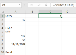
■ value2… (optional argument) – You can add up to 255 additional items, cell references, or ranges where you want to count numeric values.Using the COUNT Function to Count Cells Containing Numeric Data
To count all the cells that contain numbers, use the COUNT function. Blank cells, logical values, text, and error values are ignored.
To count the number of cells with numbers:
NOTE: This function only counts numbers and ignores everything else.
-
In cells A1:A10, enter various data (numeric and text).
-
Select cell C1 and type the following formula:
=COUNT(A1:A10) -
Press Enter.
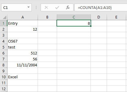
Using the COUNTA Function to Count Cells Containing Data
To count all non-empty cells containing any type of data in a range or table, use the COUNTA function.
Syntax:
=COUNTA(value1, value2, …)
value1, value2, …: 1 to 30 arguments representing the values to count.To count all cells containing data:
-
In cells A1:A10, enter any type of data (numbers and text).
-
Select cell C1 and type the formula:
=COUNTA(A1:A10) -
Press Enter.
Using COUNTA and COUNT to Count Cells Containing Text
To count all cells that contain text values, combine functions in a formula.
The number of cells with any type of data is counted with COUNTA.
Numeric cells are counted with COUNT.
Simply subtract the result of COUNT from COUNTA for the same range to get the number of text cells.To count only cells with text:
-
In cells A1:A10, enter any data (numbers and text).
-
Select cell C1 and type the following formula:
=COUNTA(A1:A10) - COUNT(A1:A10) -
Press Enter.
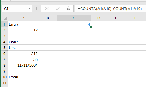
NOTE: The COUNTA function does not count empty cells.
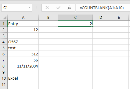
Using the COUNTBLANK Function to Count Empty Cells
Sometimes, it is useful to determine how many cells in a range are empty.
You can use the COUNTBLANK function to count all empty cells in a range.Syntax:
=COUNTBLANK(range)
range: The range in which to count the blank cells.To count all empty cells in a given range:
-
In cells A1:A10, enter data (numeric and text), leaving some cells blank.
-
Select cell C1 and type the formula:
=COUNTBLANK(A1:A10) -
Press Enter.
Using COUNTA to Determine the Last Filled Row
In this example, you need to determine the last row that has been filled in a worksheet.
If all the cells in a column contain data and are not empty, you can use the COUNTA function.
Set the range to the entire column to count all filled cells.To determine the last filled row:
-
In cells A1:A10, enter data (numbers and text).
-
Select cell B1 and type the formula:
=COUNTA(A:A) -
Press Enter.
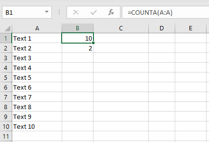
NOTE:
To determine the last filled column in a worksheet, use the formula=COUNTA(1:1), as shown in cell B2.-