Votre panier est actuellement vide !
Étiquette : practical_excel
Absolute, Relative, and Mixed Cell References in Excel
A worksheet in Excel is made up of cells. These cells can be referenced by specifying the row number and column letter. For example,
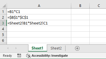
A1refers to the first row (indicated by 1) and the first column (indicated by A). Likewise,B3refers to the third row and the second column.The power of Excel lies in the fact that you can use these cell references in other cells when creating formulas. There are three types of cell references that you can use in Excel:
- Relative cell references
- Absolute cell references
- Mixed cell references
Understanding these different types of cell references will help you work more efficiently with formulas and save time (especially when copying and pasting formulas).
Relative Cell References
Let’s take a simple example to explain the concept of relative cell references in Excel. Suppose we have the following data set:
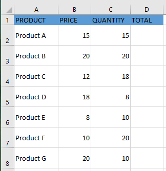
To calculate the total for each item, we need to multiply the price of each item by its quantity. For the first item, the formula in cell
D2would be=B2*C2(as shown below):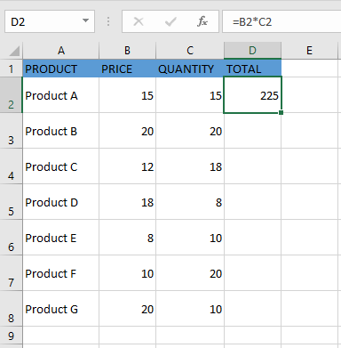
Now, instead of entering the formula for each cell individually, you can simply copy the formula from cell
D2and paste it into all the other cells (D3:D8) using the fill handle. When you do this, you’ll notice that the cell references adjust automatically to refer to the corresponding rows. For example, the formula inD3becomes=B3*C3, and inD4, it becomes=B4*C4.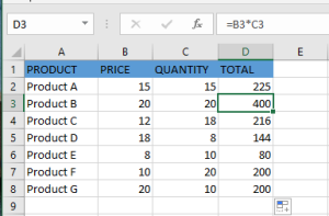
These cell references that adjust when the formula is copied are called relative references in Excel. Relative cell references are useful when you want to create a formula for a range of cells and have the reference adjust automatically for each row or column. In such cases, you can create the formula once and copy-paste it across the range.
Absolute Cell References
Unlike relative references, absolute cell references do not change when you copy the formula to other cells. For example, suppose you have the dataset below and need to calculate the commission for the total sales of each item. The commission rate is 20% and is listed in cell
G1.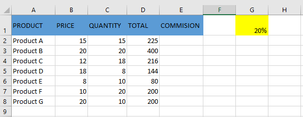
To calculate the commission amount for each item’s sales, use the following formula in cell
E2and copy it to the other cells:=D2*$G$1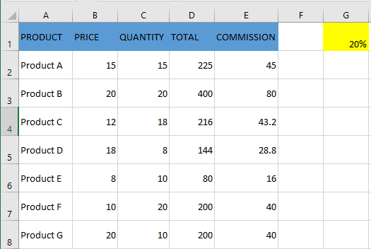
Notice that there are two dollar signs
$in the commission cell reference$G$1. What does the dollar sign do?A dollar sign, when added before the column letter and row number, makes the reference absolute (i.e., it prevents the row and column from changing when the formula is copied). For example, in the case above, when the formula is copied from
E2toE3, it changes from=D2*$G$1to=D3*$G$1. Notice that whileD2changes toD3,$G$1remains the same. This is because both the columnGand the row1are locked with the$symbol.Absolute cell references are useful when you don’t want a reference to change when copying formulas. This is often the case when using a fixed value in a formula (such as a tax rate, commission rate, number of months, etc.).
While you could hardcode this value into the formula (e.g., use
20%instead of$G$1), using a cell reference allows you to update the value later. For example, if the commission rate changes from 20% to 25%, you can simply update the value in cellG1, and all formulas will update automatically.Mixed Cell References
Mixed cell references are a bit more complex than relative and absolute references. There are two types of mixed references:
- The row is locked while the column changes when the formula is copied.
- The column is locked while the row changes when the formula is copied.
Let’s see how this works with an example.
Below is a dataset where you need to calculate three levels of commission based on the percentage values in cells
E2,F2, andG2.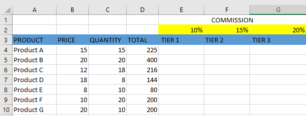
You can now use the power of mixed references to calculate all these commissions with a single formula. Enter the following formula in cell
E4and copy it across all relevant cells:=$B4*$C4*E$2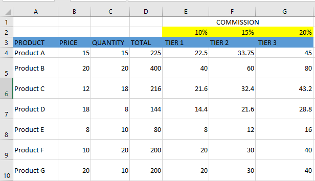
The formula above uses two types of mixed references (one with the row locked, one with the column locked). Let’s analyze each reference:
$B4(and$C4) – The dollar sign is placed before the column letter but not before the row number. This means the column is fixed, but the row will adjust when copying the formula down. For example, when copying fromE4toF4, the column staysBandC, but the row changes if you copy downwards.E$2– The dollar sign is placed before the row number but not the column. This means the row is fixed, but the column will adjust when copying the formula horizontally. For example, copying fromE4toF4changesE$2toF$2.
How to Change a Reference from Relative to Absolute (or Mixed)
To change a reference from relative to absolute, add a dollar sign before both the column letter and the row number. For example,
A1(relative) becomes$A$1(absolute).If you only have a few references to change, you can manually edit them in the formula bar or by selecting the cell and pressing
F2.However, a faster way is to use the F4 keyboard shortcut. When a cell reference is selected (either in the formula bar or in edit mode), pressing
F4toggles the reference type:- Press
F4once →A1becomes$A$1(absolute) - Press
F4twice →A1becomesA$1(row locked) - Press
F4three times →A1becomes$A1(column locked) - Press
F4four times → reference returns toA1(relative)
Alternative Text to Objects for Accessibility in Excel
Alternative text allows screen readers to capture the description of an object and read it aloud, providing support to people with visual impairments.
To add alternative text to an object in Microsoft Excel:
- Open your worksheet and insert an object (via Insert > Picture).
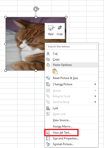
- Select the object.
- Right-click on the object, then choose Edit Alt Text from the context menu.
Unlike the Alt Text pane in Word or PowerPoint, Excel does not include the “Generate a description for me” option. You’ll need to write the description manually.
As a general rule, keep the alt text brief and descriptive.
You can omit unnecessary phrases such as « image of » or « photo of », as screen readers already indicate that the object is an image.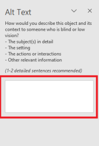
Modify Object Properties in Excel
Charts and objects inserted into your workbooks have properties that you can update to control their behavior.
You can also add alternative text so that your worksheet is accessible to people who have difficulty reading text and graphics on screen.Once an object is inserted, you can adjust its properties to control how it moves and resizes, whether it prints, and whether it is locked.
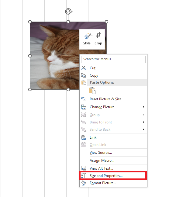
Steps to modify an object’s properties:
- Right-click on the image or object.
- Select Size and Properties. The Format Picture pane will appear on the right.
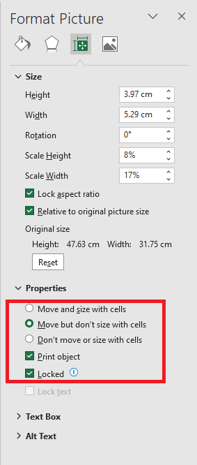
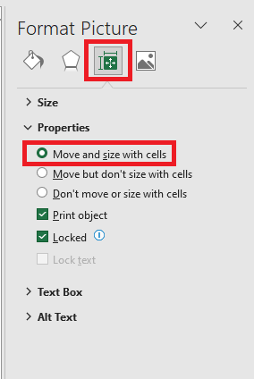
- Expand the Properties section.
- Choose a property option:
- Move and size with cells:
If you resize the surrounding cells, the object will move with them. If you resize the cells that the object overlaps, it will also stretch accordingly. - Move but don’t size with cells:
The object moves with the surrounding cells if they are resized, but it will not stretch. It keeps its original size unless manually resized from the Format tab. - Don’t move or size with cells:
The object retains the same size and position even if the surrounding cells are resized.
Inserting Images in Excel
Although Microsoft Excel is primarily used as a calculation program, in some situations, you may want to store images with your data and associate an image with a specific piece of information.
For example:- A sales manager creating a product spreadsheet might want to include a column with product images,
- A real estate agent might want to add pictures of various buildings,
- A florist will likely want photos of flowers in their Excel database.
How to Insert an Image in Excel
All versions of Microsoft Excel allow you to insert images stored anywhere on your computer or a connected network. You can also add images from web pages or online storage such as OneDrive, Facebook, or Flickr.
Insert an Image from Your Computer
Inserting an image from your computer into an Excel worksheet is simple. Just follow these 3 quick steps:
- In your Excel worksheet, click where you want to place the image.
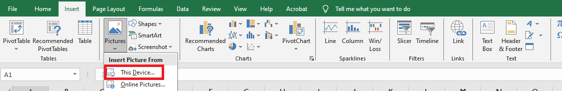
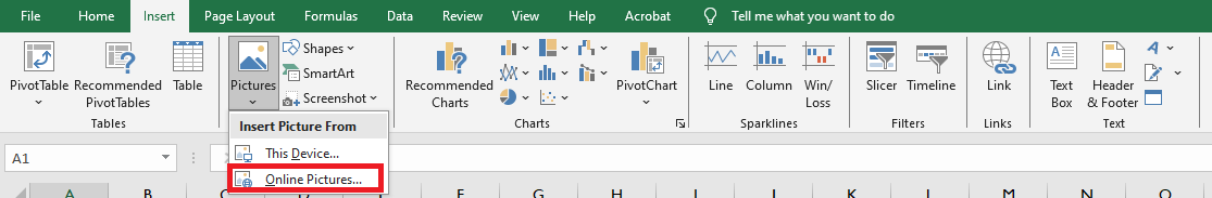
- Go to the Insert tab, in the Illustrations group, click Pictures, then choose This Device…
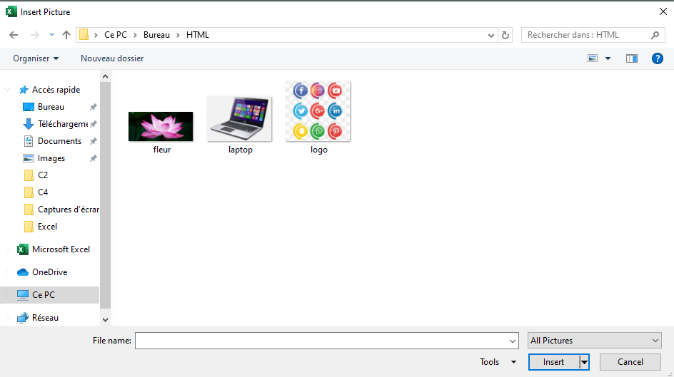
- In the Insert Picture dialog box that opens, locate and select the image you want, then click Insert.
The image will appear near the selected cell, specifically with its top-left corner aligned with the cell’s top-left corner.
To insert multiple images at once, hold down the Ctrl key while selecting the images, then click Insert.
You can now reposition or resize your image, or even lock it to a specific cell so that it resizes, moves, hides, or filters along with the associated cell.
Insert an Image from the Web, OneDrive, or Facebook
You can also add images from web sources using Bing Image Search. Here’s how:
- On the Insert tab, click Online Pictures.
- A window will appear. Type what you’re looking for in the search bar and press Enter.
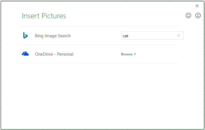
- From the search results, click to select your preferred image, then click Insert.
You can also select multiple images to insert all at once.
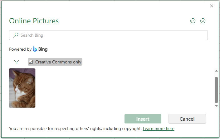
If you’re looking for something specific, use the filters at the top of the search results to sort by size, type, color, or license.
In addition to Bing search, you can insert images stored on OneDrive, Facebook, or Flickr.
Paste an Image from Another Program
The simplest way to insert an image from another application into Excel is:
- Copy an image from another app (e.g., Paint, Word, or PowerPoint) using Ctrl + C.
- Return to Excel, select the desired cell, and press Ctrl + V to paste the image.

How to Insert an Image into a Cell
Typically, an image in Excel “floats” on a separate layer.
To insert an image into a cell (so it behaves like part of the cell):- Resize the inserted image to fit into a cell. Resize or merge cells if necessary.
- Right-click the image and select Format Picture…
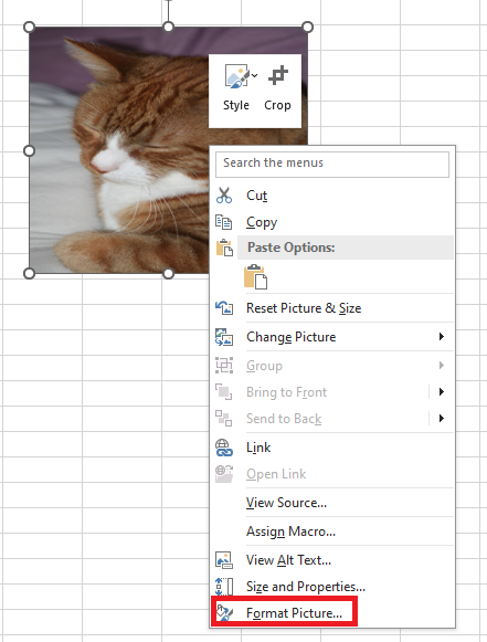
- In the Format Picture pane, go to the Size & Properties tab and select Move and size with cells.
Repeat for each image. You can even place multiple images in a single cell if needed.
As a result, your Excel sheet will be neatly organized with images linked to specific data.
When you move, copy, filter, or hide the cells, the images will follow accordingly.Embed an Image in a Header or Footer
To insert an image in a worksheet’s header or footer:
- Go to the Insert tab, in the Text group, click Header & Footer.
- Click in the Left, Center, or Right header section. For footers, click “Add Footer” and select a section.
- Under the Header & Footer tab, in the Header & Footer Elements group, click Picture.
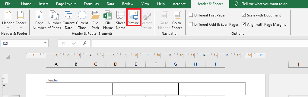
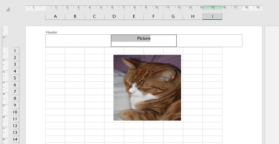
- In the dialog box, browse and insert your desired image. A placeholder will appear; click outside the header to display the image.
Insert Data from Another Sheet as an Image
Excel allows you to copy content from one sheet and insert it as an image into another sheet.
This is useful for summary reports or printing data from multiple sheets.You can do this using:
- Copy as Picture: inserts a static image.
- Camera Tool: inserts a dynamic image that updates with changes.
Copy as Picture
- Select the data, charts, or objects.
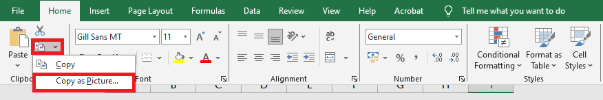
- On the Home tab, in the Clipboard group, click the dropdown next to Copy, then click Copy as Picture…
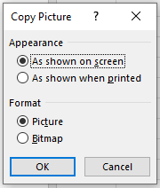
- Choose As shown on screen or As shown when printed, then click OK.
- Go to the destination sheet, click where you want the image, and press Ctrl + V.
Use the Camera Tool (Dynamic Image)
To activate the Camera tool:
- Go to File > Options > Quick Access Toolbar.
- Under Choose commands from, select Commands Not in the Ribbon.
- Find and select Camera, then click Add > OK.
- The Camera icon now appears on the toolbar.

To use it:
- Select the cell range to capture.
- Click the Camera icon.
- Click the destination location in another sheet.
This creates a “live” image that updates automatically with changes in the source cells.
How to Modify an Image
Once inserted, you may want to reposition, resize, or style the image. Below are some common operations.
Copy or Move an Image
To move an image:
- Select it, then drag it with your mouse (the pointer turns into a four-sided arrow).
- Hold Ctrl and use arrow keys to move it pixel-by-pixel.

- To move to another sheet or workbook, press Ctrl + X, then Ctrl + V in the new location.
To copy an image:
- Select it and press Ctrl + C, then Ctrl + V to paste.
Resize an Image
The easiest way to resize an image is by dragging the corner handles.
To preserve the aspect ratio, drag from a corner.
Alternatively, use the Picture Tools > Format tab to enter exact width and height (in inches).
Entering one value will automatically adjust the other proportionally.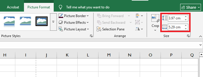
Change Image Colors and Styles
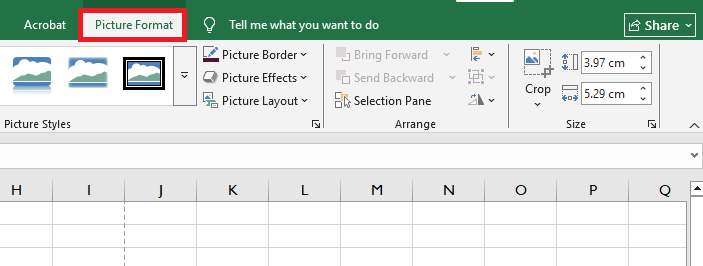
Excel offers many built-in effects for images. To access them, select the image and go to the Format tab under Picture Tools.
Useful options:
- Remove Background
- Corrections (brightness, contrast, sharpness)
- Color (tone, saturation, recoloring)
- Artistic Effects (paint/sketch-like)
- Picture Styles (borders, 3D effects, shadows)
- Picture Border
- Compress Pictures (to reduce file size)
- Crop
- Rotate (flip vertically/horizontally)
To restore original format and size, click Reset Picture.
Replace an Image
To replace an image:
- Right-click the image, select Change Picture, choose the new source (from file or online), select the image, and click Insert.
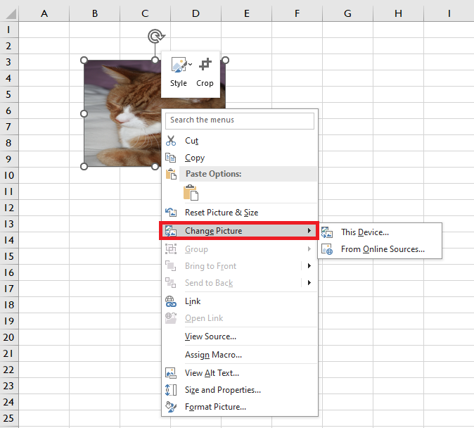
The new image will retain the same formatting and position as the previous one.
Delete an Image
To delete a single image:
- Select it and press Delete.
To delete multiple images:
- Hold Ctrl while selecting multiple images, then press Delete.
To delete all images:
- Press F5 to open the Go To dialog.
- Click Special…, select Objects, and click OK.
- All objects (images, shapes, WordArt, etc.) will be selected. Press Delete to remove them.
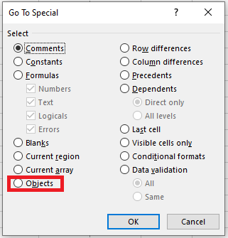
Be careful: this selects all objects on the sheet—ensure no important items are included before deleting.
Inserting Text Boxes and Shapes in Excel
Inserting Text Boxes
Unlike cell text, a text box can be placed anywhere in Microsoft Excel as a label or a comment on the worksheet in a separate window.
To insert a text box:- Go to the Insert tab, then find the Text Box button in the Text section.
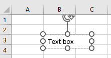
- You can now draw a text box—your cursor will immediately change to an inverted cross.
- Click anywhere on the worksheet to create the text box and type inside it.
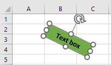
You can change the background color of the text box, as well as the font, size, and color of the text it contains.
To move it, press and hold the mouse to drag the dotted border to your desired location. You can also rotate it using the rotation handle above the box.
Insert a Text Box Using the Shapes Menu
You can also insert a text box through the Shapes menu:
- In the ribbon, go to Insert > Illustrations > Shapes > Text Box.
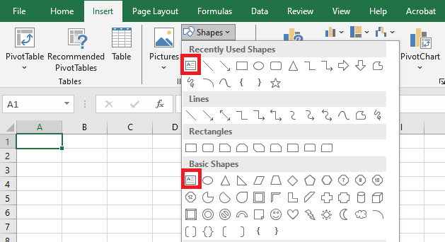
- The Text Box icon will also appear in the Recently Used Shapes group if you’ve inserted one recently.
How to Remove the Text Box Border
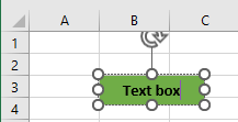
- Click the text box. A new tab will appear in the ribbon: Shape Format.
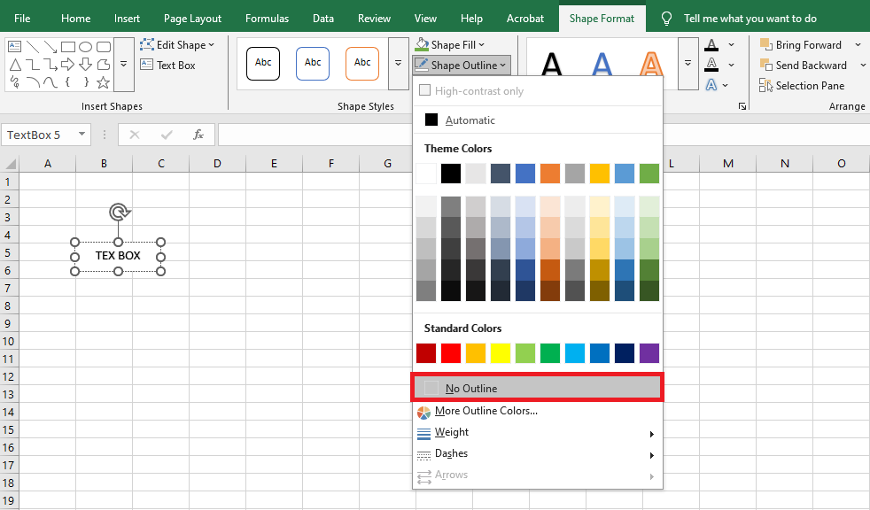
- Go to Shape Format > Shape Outline > No Outline to remove the default border.
You can also use Shape Fill to change the fill color and Text Fill to change the text color.
Using Shapes
Excel gives access to various customizable graphic objects called Shapes. You may want to insert shapes to create simple diagrams, display text, or add visual interest.
Keep in mind: Shapes can add unnecessary clutter. Use them sparingly—they should enhance, not dominate.
Inserting a Shape
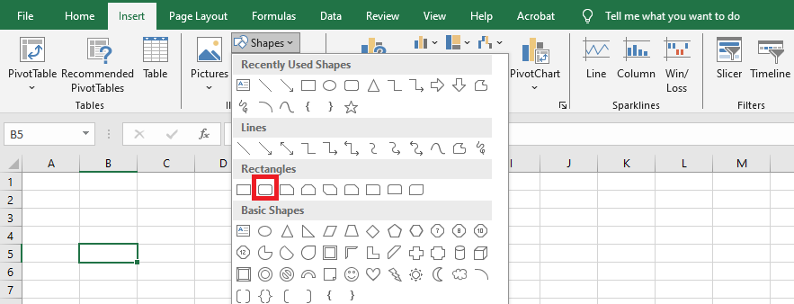
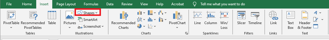
To add a shape:
- Go to Insert > Illustrations > Shapes to open the Shapes gallery.
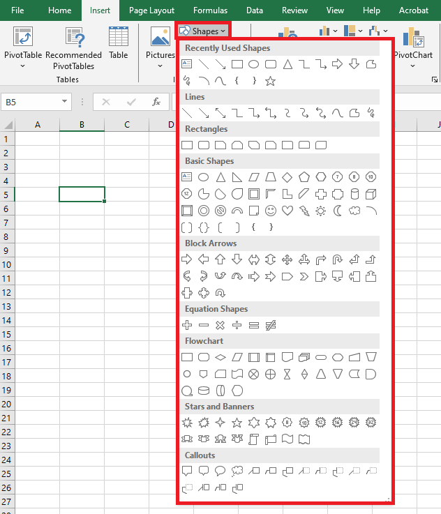
- Shapes are grouped by category, with Recently Used Shapes at the top.
To insert a shape:
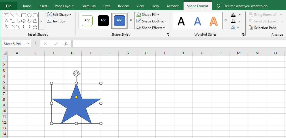
- Click a shape, then click anywhere on the sheet to place it with default size.
- Or, click and drag to define custom size and proportions.
Once placed, the shape is selected and named.
You can also insert a shape inside a chart. Just select the chart first, then insert the shape—it becomes embedded and moves/resizes with the chart.
Some shapes require special drawing:
- Freeform: Click repeatedly to create lines, or click-and-drag for irregular shapes. Double-click to finish.
- Curve: Click multiple times.
- Scribble: Drag the mouse pointer freely; closing the shape will make it filled.
Tips:
- Shapes have names (e.g., “Rectangle 1”). You can rename them in the Name Box.
- Click a shape to select it.
- Hold Shift while dragging to maintain proportions.
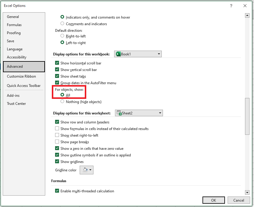
- Hide/display all objects via File > Options > Advanced > Display options for this workbook.
Modifying Shapes
To modify a shape:
- Click to select it.
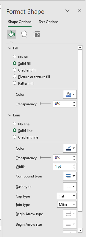
- Right-click and choose Format Shape.
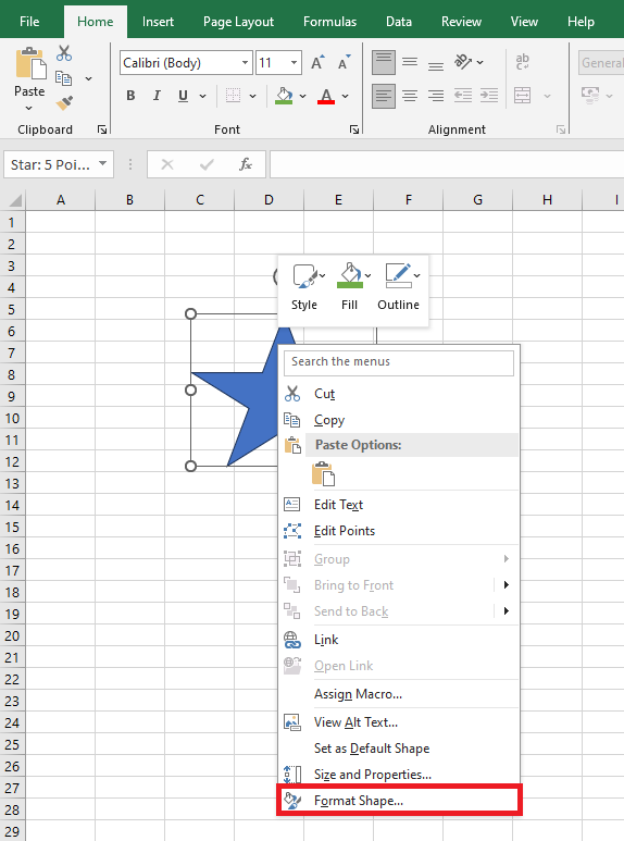
- The Format Shape pane appears on the right. You can adjust fill type and color, border color and thickness, add shadows, glow, reflections, and more.
Using Shapes as Macro Buttons
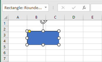
You can use a shape (e.g., a rounded rectangle) as a macro button:
- Go to Insert > Illustrations > Shapes, then pick a shape.
- Click the sheet to insert the shape.
- The shape appears with a default name.
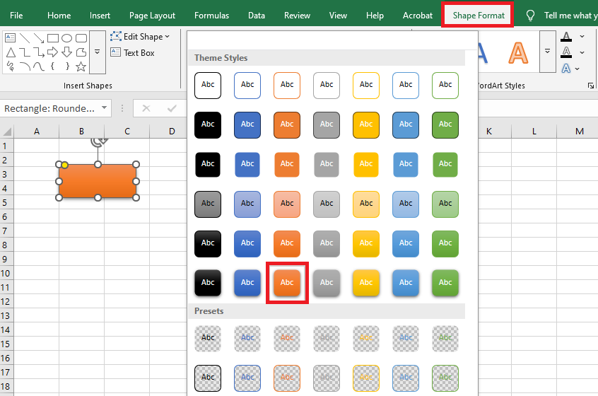
To make it look like a button:
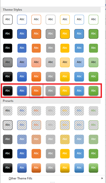
- Select the shape, go to Shape Format, then Shape Styles > More.
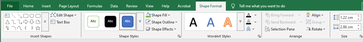
- Choose a style like Intense Effect (for a 3D shadow).
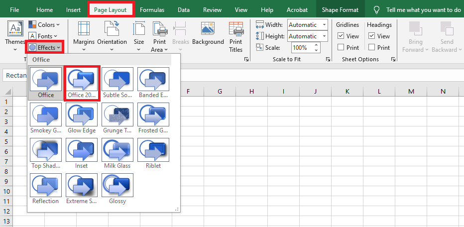
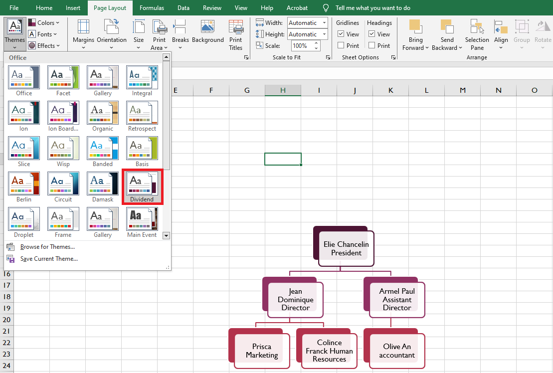
- For consistent styling, go to Page Layout > Themes > Effects > Office 2007-2010.
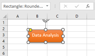
To add a label:
- Right-click the shape, type the button text, then click the border to exit text-edit mode.
- Format the text (bold, size, alignment) via the Home tab.
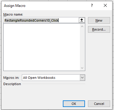
To assign a macro:
- Right-click the shape > Assign Macro…
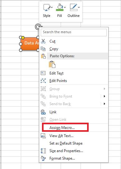
- Choose the macro from the list > Click OK.
SmartArt Graphics
SmartArt lets you visualize information with graphics rather than plain text. It offers various styles for different concepts.
To insert a SmartArt graphic:
- Place the cursor where you want it to appear.
- Go to Insert > Illustrations > SmartArt.
- A dialog opens: select a category, pick a graphic,
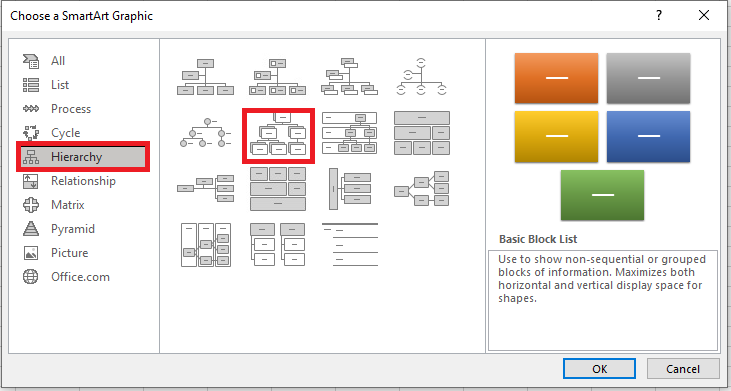
then click OK.

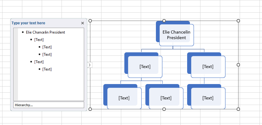
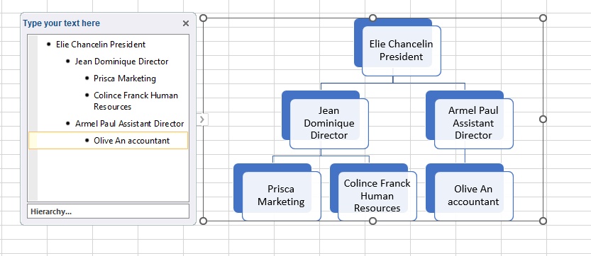
To add text:
- Select the SmartArt. The SmartArt pane opens on the left.
- Enter text next to each bullet. The text appears inside the shapes.
- Press Enter to add more bullets and shapes. To delete, remove bullets.
Alternatively, click a shape to type directly. For complex graphics, the pane is faster.
Editing SmartArt Layout
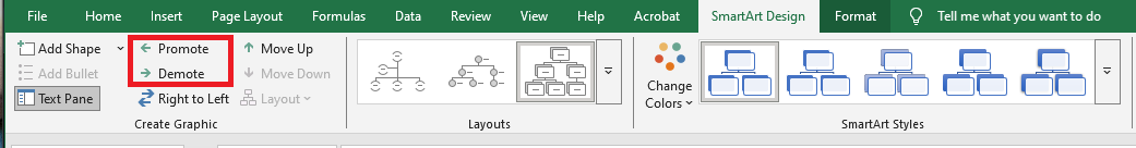
To add a shape:
- Select the SmartArt and go to the Design tab.

- Select a nearby shape.
- Click Add Shape, then choose:
- Add Shape Before/After (same level)
- Add Shape Above/Below (different level)
To rearrange:
- Select the SmartArt > Design tab.
- Select the shape.
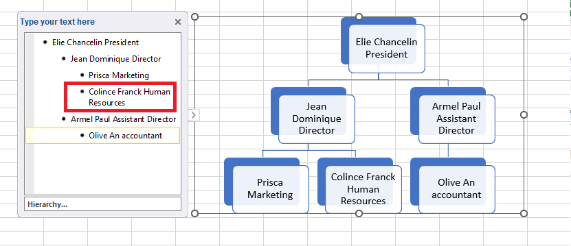
- Click Move Up/Down to change its order—subordinate shapes move with it.
Customizing SmartArt
Use the Design and Format tabs to customize:
- Click Change Colors to use a color scheme from your document’s theme.
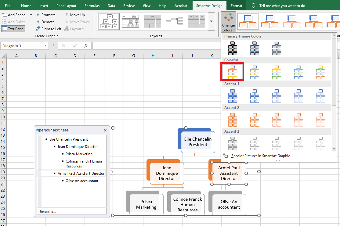
- Color sets vary by theme.
Changing SmartArt Layout
To modify the layout:
- Select the SmartArt > Design tab.
- In the Layouts group, click the dropdown for more layouts.
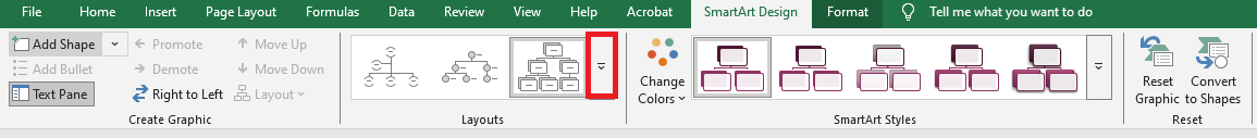
- Pick a new layout. If it’s too different, some text may not display
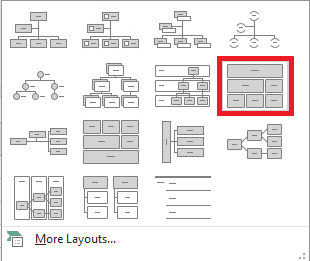
Verify before confirming.

WordArt
You can enhance a spreadsheet by formatting cells and fonts, or by using WordArt—a powerful feature in Excel. For instance, you might use it to style a range header instead of regular text.
Inserting WordArt
To insert WordArt:
- In the worksheet, go to the Insert tab.
- Click Text > WordArt.
- A dropdown appears with multiple styles—choose one.
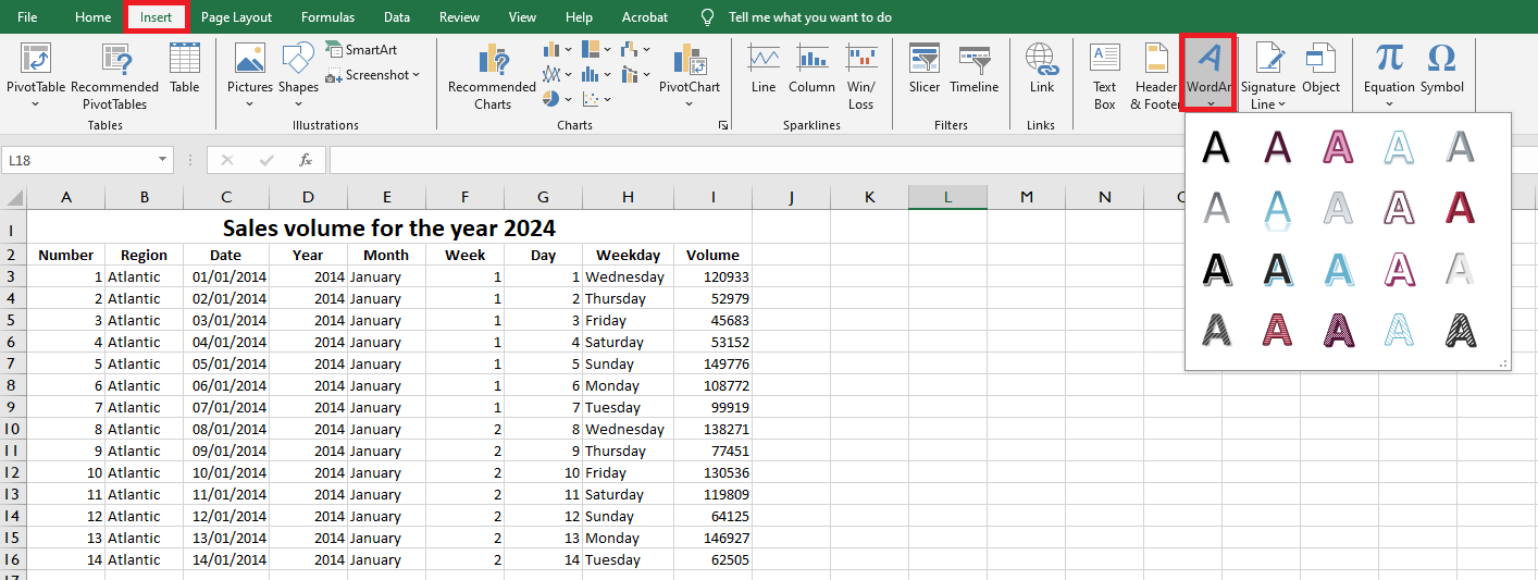
- Type your text in the box.

- Click anywhere else on the sheet to complete.
Editing WordArt
After insertion:
- Move it to the right place (e.g., top of the sheet for a header).
- Clicking it activates Drawing Tools.
- Under Shape Styles, pick a default or custom style.
- Under WordArt Styles, format the text’s color, outline, and effects.
The result is often more visually appealing than regular font formatting—consider using WordArt next time to enhance your spreadsheet’s appearance.
Moving Charts to a Chart Sheet in Excel
When we create a chart using data on a worksheet, by default, the chart is created on the same sheet and can be moved using the mouse. However, sometimes it’s better to have a standalone chart that fits entirely on its own sheet and remains fixed in place. In this article, we’ll learn how to move a chart from a worksheet to a new chart sheet.
Steps to move the selected chart to a new chart sheet:
- Select the chart and go to the Design tab.

- You will see the Move Chart icon on the far-right corner of the ribbon in Excel. Click it.
- In the Move Chart dialog box, click the New sheet radio button. Change the chart name if desired.
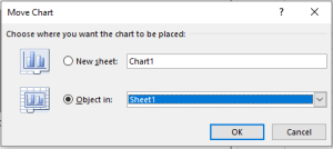
- Click OK. The chart will be moved to a new chart sheet.
In a chart sheet, the chart is properly fitted and fixed in place, but you can still perform all chart-related tasks. This sheet belongs to the workbook. The chart is designed to fit this sheet, making it ideal for data presentation.
You can also move other charts onto the same sheet, but those charts will float while the first chart remains as the sheet background.
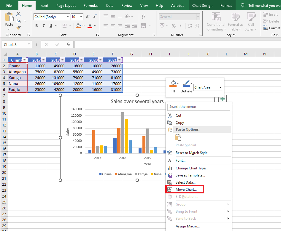
You can also move the chart by right-clicking on it. When you right-click the chart, you will see an option Move Chart…. Click it. The same Move Chart dialog box will appear.
Moving a chart from one worksheet to another
If you want to move the chart to another standard worksheet, select the Object in option. From the dropdown list, select the desired worksheet name. Press OK. The chart will be moved. The same can be done using standard cut and paste.Moving a chart from a chart sheet back to a worksheet
On the chart sheet, right-click the chart. Click Move Chart. Select Object in and choose the desired sheet from the dropdown list.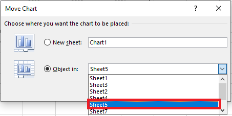
Press OK. The chart will be returned to the standard worksheet. The chart sheet will be deleted.
Searching for Data in a Workbook in Excel VBA
Find or Replace Text and Numbers in a Worksheet
The Find and Replace functions in Excel are used to search for a number or a string of text within a worksheet or an entire workbook. You can use them either to locate the item for reference purposes or to replace it with another value. You can include wildcards such as question marks (?), tildes (~), asterisks (*), or numbers in your search terms. Searches can be performed across rows and columns, within comments or cell values, and across worksheets or entire workbooks.
Basic Find
To find an occurrence of a specific value in a worksheet:
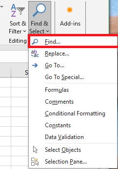
Click on the Find & Select icon (located in the Editing group on the Home tab of the Excel ribbon), then select the Find option.
NOTE:
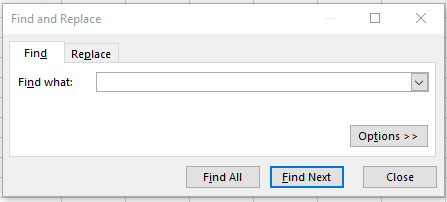
The keyboard shortcut for this is Ctrl + F.The Find and Replace dialog box will appear with the Find tab selected, as shown below:
-
In the dialog box:
-
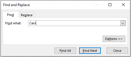
Type the text or numeric value you want to find in the Find what field.
-
Click the Find Next button.
This will take you to the next occurrence of the desired value in the current worksheet.
Find All
If you want to locate all occurrences of a specific value, click the Find All button in the Find and Replace dialog box. This displays a list of all instances of your search term, as shown in Figure.
Clicking any value in the list will take you to the corresponding cell in your worksheet.
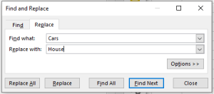
Basic Replace
To replace one or more occurrences of a specific value in an Excel worksheet:
Click the Find & Select button (located in the Editing group on the Home tab), then choose the Replace… option.
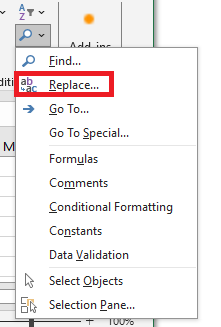
The Find and Replace dialog box will open with the Replace tab selected, as illustrated below:
NOTE:
The keyboard shortcut to access this feature is Ctrl + H.In the dialog box:
a. Type the text you want to find in the Find what field.
b. Type the text you want to replace it with in the Replace with field.
c. Click the Find Next button. This will take you to the first occurrence of the search text.
d. To replace the current instance of the search text with the specified replacement text, click the Replace button. The text will be replaced, and you will be taken to the next occurrence.NOTE:
You can leave the Replace with field empty if you simply want to remove all instances of the search text (i.e., replace them with nothing).If you’re certain that you want to replace all occurrences of the search text with the replacement text (without reviewing each case individually), simply click Replace All in the dialog box.
NOTE:
You can use wildcard characters (question mark ?, asterisk *, tilde ~) in your search criteria.-
Use the question mark (?) to find any single character. For example,
s?twill match “sat” and “set”. -
Use the asterisk (*) to find any number of characters. For example,
t*s*will match “triste” and “saturé”. -
Use the tilde (~) followed by
?,*, or~to search for actual question marks, asterisks, or tildes. For example,fy91~?will find “fy91?”.
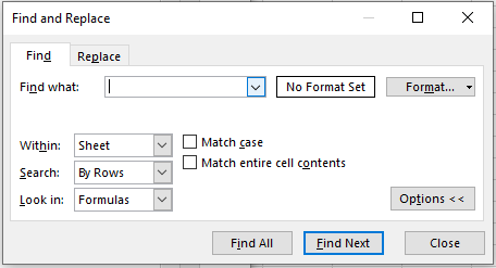
Advanced Search Options
The Find and Replace command can be refined using several options, which can be displayed by clicking the Options button in the Find and Replace dialog box.
Clicking the Options button expands the dialog box, as shown below:
Most of these options are also available in the Replace tab of the dialog box.
Each option is explained below:
-
Within: Allows the user to choose whether the search should be performed in the active worksheet only, or throughout the entire current workbook.
-
Search: Determines the direction Excel uses to perform the search:
-
If set to By Rows, Excel searches each row before moving to the next row.
-
If set to By Columns, Excel searches each column before continuing to the top of the next column.
-
-
Look in: Lets the user decide what Excel should search:
-
Formulas: If a cell contains a formula, Excel searches the formula text—not the result.
-
Values (not available in the Replace tab): Excel searches the result of the formula, not the formula itself.
-
Comments (not available in the Replace tab): Only cell comments are searched; cell contents are ignored.
-
-
Match case: Allows the user to make the search case-sensitive.
-
If unchecked (default), the search is not case-sensitive.
-
If checked, the search will distinguish between uppercase and lowercase letters.
-
-
Match entire cell contents: Lets the user specify whether to match the entire content of a cell or just part of it.
-
If unchecked (default), Excel will find the search term even if it’s just part of a cell’s content.
-
If checked, Excel will only return matches where the entire cell exactly matches the search term.
-
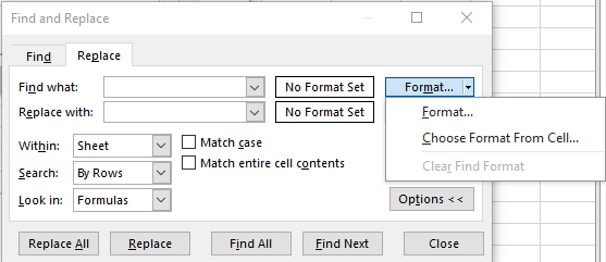
Find and Replace a Formatting Style
In the Find and Replace dialog box, you’ll also find the Format… button. This allows you to specify a format you want to search for, and optionally, a format to replace it with.
Note: If you specify both a format and a text search value, Excel will only find cells that match both the specified format and text.
In the Find Format dialog, you can define formatting based on:
-
Number
-
Alignment
-
Font
-
Border
-
Fill
-
Protection
To search for specific formatting:
-
In the Find tab of the Find and Replace dialog box, click Format, then click Choose Format From Cell under the dialog box.
-
When the pointer turns into an eyedropper, click on the cell you want to base your search on.
-
In the Find and Replace dialog box, click Find Next.
How to Clear a Formatting Style from Find and Replace
If you want to remove a previously specified formatting style from the Find and Replace dialog box:
Click the arrow next to the Format… button and select Clear Find Format.
-
Copying and Moving a Worksheet in Excel
There are many situations where you may need to create a new worksheet based on an existing one or move a sheet tab from one Excel file to another. For example, you may want to back up an important worksheet or create multiple copies of the same sheet for testing purposes. Fortunately, Excel provides a few simple and quick methods to duplicate worksheets.
Copy a Worksheet in Excel
Excel offers three built-in methods to duplicate worksheets. Depending on your preferred working style, you can use the ribbon, the mouse, or the keyboard.
Method 1: Copy the Worksheet by Dragging
Normally, you use drag-and-drop to move items from one place to another. But this method also works to copy worksheet tabs and is actually the fastest way to duplicate a sheet in Excel.
Simply click on the tab of the worksheet you want to copy, hold down the Ctrl key, and drag the tab to the desired location.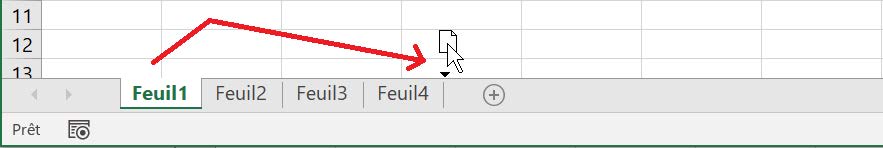
Method 2: Duplicate a Sheet Using Right-Click
Here’s another easy way to duplicate a sheet in Excel:
-
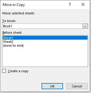
Right-click on the sheet tab and select Move or Copy from the context menu. This opens the Move or Copy dialog box.
-
Under Before sheet, choose where you want to place the copy.
-
Check the Create a copy box.
-
Click OK.
For example, this is how you can make a copy of Sheet1 and place it before Sheet3.

Method 3: Copy a Sheet Using the Ribbon
The Ribbon includes all Excel functionalities—you just need to know where to find them. To copy a sheet using the ribbon:
-
Go to the Home tab.
-
Click Format in the Cells group.
-
Select Move or Copy Sheet…
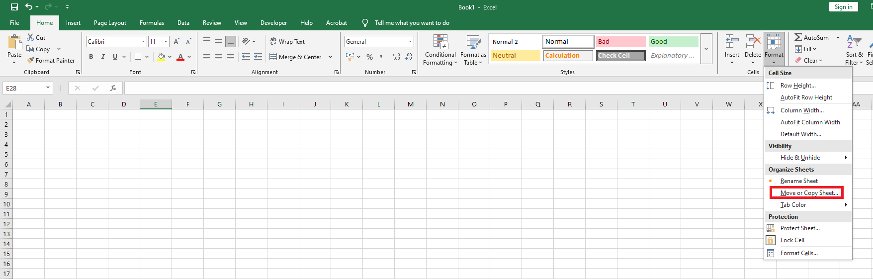
The Move or Copy dialog box appears. Follow the same steps as in the previous method.
Copy a Worksheet to Another Workbook
The most common way to copy a worksheet to another workbook is as follows:
-
Right-click the tab of the sheet you want to copy, then click Move or Copy…
-
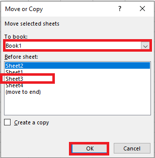
In the Move or Copy dialog box, do the following:
-
Under To book, select the target workbook. To place the copy in a new workbook, select (new book).
-
Under Before sheet, specify where to place the copied sheet.
-
Check the Create a copy box.
-
Click OK.
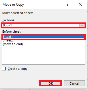
NOTE:
Excel only displays open workbooks in the To book drop-down list, so make sure to open the destination file before copying.Aside from this traditional method, there is another way to achieve the same result.
Copy a Sheet to Another Workbook by Dragging
If Excel allows duplicating a sheet within the same workbook by dragging, why not try using this method to copy a sheet to another workbook? You just need to view both files at the same time. Here’s how:
-
Open both the source and target workbooks.
-
On the View tab, in the Window group, click View Side by Side. This arranges the two workbooks horizontally.
In the source workbook, click the sheet tab you want to copy, hold Ctrl, and drag the sheet into the target workbook.
Copy Multiple Sheets in Excel
All techniques that work to duplicate a single sheet can also be used to copy multiple sheets. The key is to select multiple worksheets. Here’s how:
-
To select adjacent sheets, click the first sheet tab, hold Shift, then click the last tab.
-
To select non-adjacent sheets, click the first sheet tab, hold Ctrl, and click the other tabs one by one.
With multiple sheets selected, do one of the following:
-
Right-click one of the selected tabs and choose Move or Copy.
-
Press Ctrl and drag the tabs to the desired location.
-
From the Home tab, click Format > Move or Copy Sheet.
Copy a Worksheet with Formulas
In most cases, copying a worksheet with formulas works the same as copying any other sheet. Formula references adjust automatically in a way that works well for most scenarios.
-
When copying a sheet within the same workbook, formulas refer to the copied sheet unless external references point to another sheet or file.
Before copying:
=[Workbook1]Sheet2!B1*[Workbook1]Sheet2!C1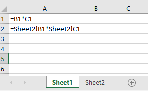
After copying:=Sheet2!B1*Sheet2!C1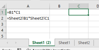
-
When copying a worksheet to another workbook, formula references behave as follows:
-
References within the same sheet (relative or absolute) point to the copied sheet in the target workbook.
-
References to other sheets in the original workbook still point to the original workbook.
You’ll notice this by the workbook name (e.g.,[Workbook1]) appearing in the formula.
-
To make copied formulas refer to a sheet with the same name in the new workbook, simply use Excel’s Replace All feature:
-
On the copied sheet, select all formulas you want to edit.
-
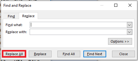
Press Ctrl + H to open the Replace tab of the Find and Replace dialog box.
-
In the Find what box, enter the name of the original workbook exactly as it appears (e.g.,
[Workbook1]). -
Leave the Replace with box empty.
-
Click Replace All.
Result:
From=[Workbook1]Sheet2!B1*[Workbook1]Sheet2!C1
To=Sheet2!B1*Sheet2!C1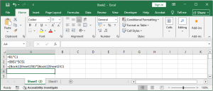
Copy Data from One Sheet to Another Using a Formula
If you don’t want to copy the entire sheet but only a portion of it, select the range of interest and press Ctrl + C to copy. Then switch to another sheet, select the top-left cell of the destination range, and press Ctrl + V to paste.
To ensure the copied data updates automatically when the original data changes, use formulas to reference another sheet.
For example, to copy data from cell A1 in Sheet1 to cell B1 in Sheet2, enter the following formula in B1:
=Sheet1!A1To copy data from another workbook, include the workbook name in brackets:
=[Workbook1]Sheet1!A1If needed, drag the formula down or across to extend the range.
Move Worksheets in Excel
Moving sheets in Excel is even easier than copying them and can be done using the same techniques.
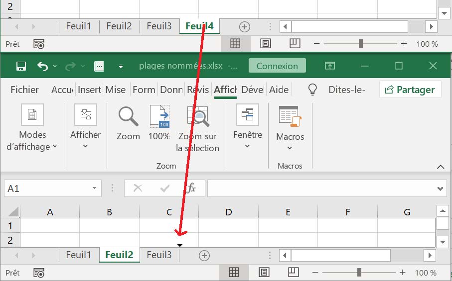
Move a Sheet by Dragging
To move one or more sheets, simply select the tab(s) and drag them to a new location.
For example, here’s how to move Sheet1 and Sheet3 to the end of the workbook.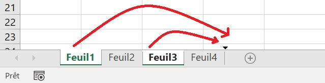
To move a sheet to another workbook, place the files side by side and drag the sheet from one file to the other.
Move a Sheet via the Move or Copy Dialog Box
Right-click the sheet tab and select Move or Copy, or go to the Home tab → Format → Move or Copy Sheet. Then:
-
To move a sheet within the same workbook, choose the target location under Before sheet, and click OK.
-
To move a sheet to another workbook, select the target workbook in the To book list, choose the sheet position, and click OK.
Note: If the target workbook already contains a sheet with the same name, Excel will add a number in parentheses to the end of the moved sheet’s name. For example, Sheet3 will become Sheet3 (2).
When Move or Copy Doesn’t Work
Normally, Microsoft Excel moves and copies sheets without issue. If a worksheet cannot be moved or copied, it may be due to the following reasons:
-
Excel Table in the Sheet
You cannot move or copy a group of sheets if one of them contains an Excel table. Each of these sheets must be handled individually. -
Protected Workbook
Moving or copying sheets is not allowed in protected workbooks. To check if the workbook is protected, go to the Review tab and look at the Protect Workbook button in the Protect group. If the button is highlighted, it means the workbook is protected. Click it to unlock the workbook, then move the sheets. -
Named Ranges Conflict
When copying or moving a sheet from one workbook to another, you may see an error message saying a name already exists. This means that both the source and target workbooks have a table or range with the same name.-
If it’s just one error, click Yes to use the existing name, or No to rename it.
-
If there are many conflicts, it’s better to review all names before copying.
To do so, press Ctrl + F3 to open the Name Manager in the active workbook—here you can edit or delete names as needed.
-
-
Add a Worksheet to an Existing Workbook in Excel
When you create a new workbook, Excel includes a single worksheet that you can use to build a spreadsheet template or store data. If you want to create a new template or store a different dataset that is related to the existing data in the workbook, you can create a new worksheet to contain the new information. Excel supports multiple worksheets in a single workbook, so you can add as many worksheets as needed for your project or template. In most cases, you’ll insert a blank worksheet, but Excel also provides several built-in templates.
Insert a Blank Worksheet
To insert a blank worksheet in a workbook, go to the Home tab, navigate to the Cells group, click the Insert command, and then choose Insert Sheet.
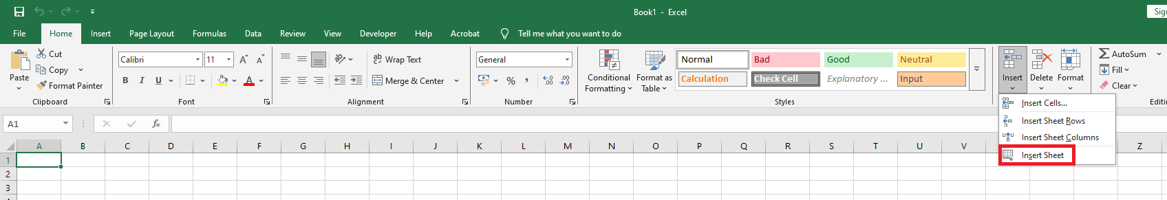
Excel inserts the worksheet.
NOTE:
You can also insert a blank worksheet by pressing Shift + F11.
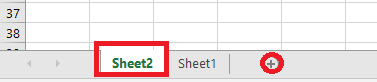
Another way to add a blank worksheet is by clicking the plus (+) icon, as shown in Figure 1.1.3-b.Insert a Worksheet from a Template
To insert a worksheet from a template, open the workbook to which you want to add the worksheet. Then, right-click on a worksheet tab and click Insert.
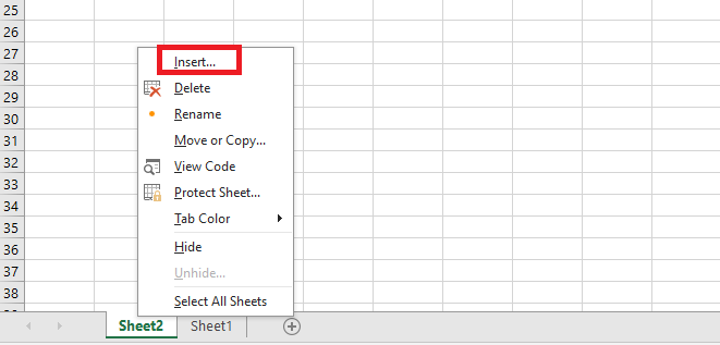
The Insert dialog box appears.
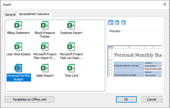
Click the Spreadsheet Solutions tab, select the type of worksheet you want to add, and then click OK.
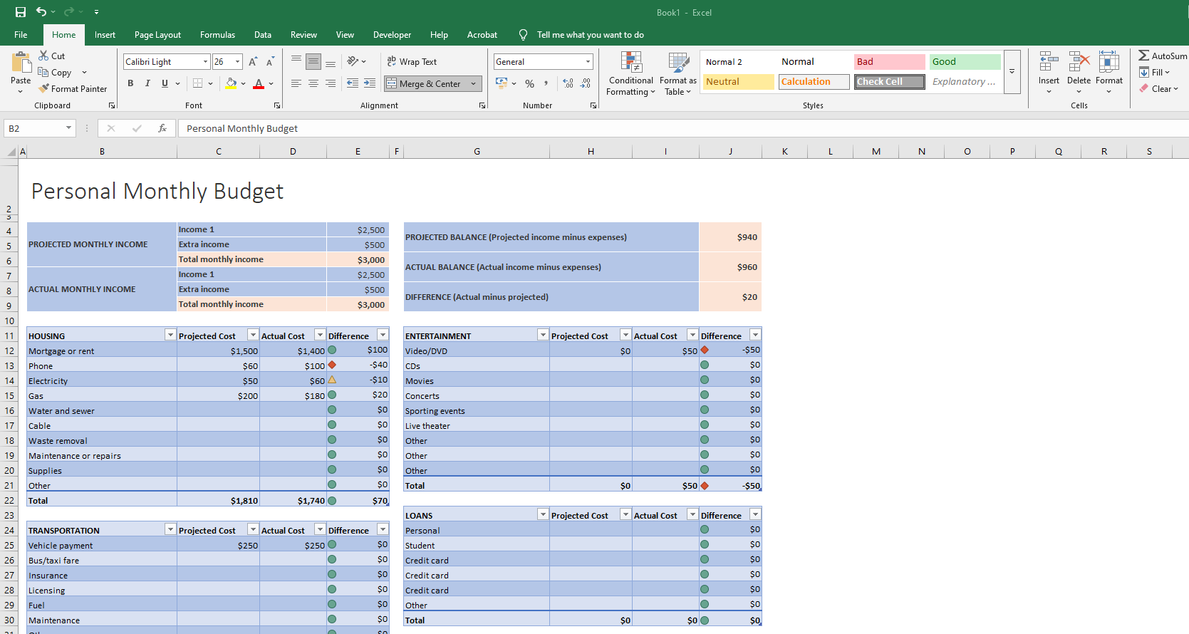
Excel inserts the worksheet.
NOTE:
You can also click Templates on Office.com to download spreadsheet templates from the web.Set the Default Number of Worksheets for New Workbooks
If you usually add worksheets to new workbooks, you can save time by configuring Excel to always include your preferred number of worksheets in every new file.
By default, Excel includes one blank worksheet in each new workbook you create. However, you may find that you typically use three, four, or more worksheets in most of your workbooks. If that’s the case, you may be wasting time adding additional sheets manually. You can save time by telling Excel how many worksheets you want in your new workbooks.
To do this, click the File tab, then Save As, and finally click Options.
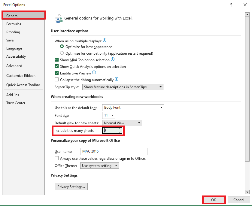
The Excel Options dialog box appears with the General tab displayed. Use the Include this many sheets box to specify how many worksheets you want in each new workbook. Click OK. From now on, whenever you create a new workbook, Excel will include the number of worksheets you’ve specified.
Importing Data from a Delimited Text File in Excel
You often need to import data into an Excel worksheet from a text file. Microsoft Excel provides a Text Import Wizard to import data from various text file formats:
■ Comma-separated files (.csv) or tab-delimited files (.txt), as shown in Figure 1.1.2-a.■ Files with fixed-width columns, where there are no delimiters between columns and data starts at fixed positions on each line (Figure 1.1.2-b).
You will often receive data in a Microsoft Word document or in a plain text file (.txt) that you need to import into Excel for analysis. To import a Word document into Excel, you must first save it as a text file.
When importing delimited data from a file, Excel evaluates the file and displays a preview of how the data will be imported. If the data exceeds certain size limits, only a portion is previewed, and a message appears indicating that the data has been truncated due to size limits. However, this does not affect the amount of data actually imported.For example, the file
importationdedonnees.docxcontains the amount of time each player played for Dallas in multiple games during a season. It also includes the performance rating for each lineup.
For example, the first two lines indicate that against Sacramento, Bell, Finley, LaFrentz, Nash, and Nowitzki were on the court together for 9.05 minutes and played at a level of 19.79 points (per 48 minutes), which is worse than the average NBA lineup.Figure 1.1.2-c: Sample data
We want to import this lineup information into Excel so that, for each lineup, the following information is listed in separate columns:
■ The name of each player
■ Minutes played by the team
■ Rating rangeA problem arises with the player Van Exel (full name: Nick Van Exel). If you choose the Delimited option and use a space to split the data into columns, “Van Exel” will occupy two columns. As a result, the numeric data for lineups that include Van Exel will appear in a different column compared to lineups that don’t include him.
To fix this, the Replace command was used in Word to change all instances of « Van Exel » to just « Exel ». Now, when Excel splits data at spaces, “Van Exel” only takes up one column.
Figure 1.1.2-d: Updated data with “Van Exel” replaced by “Exel”The key to importing data from a Word or text file into Excel is to use Excel’s Text Import Wizard. As mentioned earlier, the Word file (in this example
importationdedonnees.docx) must first be saved as a text file.To save a Word document as a .txt file (Plain Text):
- Click the File tab.
- Click Save As.
- Click Browse, then choose where to save your file.
- In the Save as type list, select Plain Text (.txt).
- Enter a name for your file, then click Save.
In the File Conversion dialog box, select Windows (Default) for the text encoding, then click OK.
Your file is now saved asimportationdedonnees.txt.Close the Word document. In Excel, to open
importationdedonnees.txt, click File, then Open, then Browse. Navigate to the .txt file folder, select All Files (*.*) in the file type list, select the file, and click Open.
You will see Step 1 of the Text Import Wizard, illustrated in the figure below:Figure 1.1.2-e: Step 1 of the Text Import Wizard
Step 1 – Key elements to consider:
- Original data type: Select Delimited when items in the text file are separated by tabs, semicolons, spaces, or other characters. Select Fixed width when all items in each column are of equal length.
- Start import at row: Enter the row number to specify where to begin the import.
- File origin: Choose the character set used in the text file. Usually, you can keep the default setting. If the text file was created using a different character set than your system, update this option to match.
- Data preview: Shows how the text appears when split into columns in the worksheet.
In our case, we choose Delimited. However, suppose you mistakenly choose Fixed width. Then Step 2 of the wizard will appear as shown in Figure 1.1.2-f, allowing you to create, move, or delete break lines. Adjusting column breaks in fixed-width mode can be imprecise and cumbersome.
Figure 1.1.2-f: Step 2 of the wizard after selecting Fixed width
If you select Delimited in Step 1, you’ll see another version of Step 2, shown in Figure 1.1.2-g.
Figure 1.1.2-g: Step 2 of the wizard after selecting Delimited
Step 2 – Key elements to consider:
- Delimiter: Choose the character that separates values in your file. If it’s not listed, check Other and type the character manually. This option is unavailable for fixed-width files.
- Treat consecutive delimiters as one: Check this if your data contains multiple consecutive delimiters or complex delimiters.
- Text qualifier: Choose the character that encloses text. When Excel sees this character, all the text between this and the next occurrence is treated as one value—even if it contains a delimiter.
For example, if the delimiter is a comma (,) and the qualifier is a double quote (« ),"Dallas, Texas"is imported as a single cell value. Without a qualifier or if you choose'as the qualifier, it may be split into two cells: « Dallas » and « Texas ».
If the delimiter character occurs inside the text qualifier, Excel ignores it; if it occurs outside, it is treated normally. - Data preview: Review the split data to ensure columns appear as desired.
In this example, we select space as the delimiter. Checking Treat consecutive delimiters as one ensures that multiple spaces don’t create unnecessary columns. It is recommended to keep Tab selected as well since some Excel add-ins rely on it.
Figure 1.1.2-h: Step 2 of the Text Import Wizard with Delimited selected
When you click Next, you reach Step 3, shown in Figure 1.1.2-i.
Figure 1.1.2-i: Step 3 of the wizard, where you can define formats for the imported data
Step 3 – Key elements to consider:
- Advanced button:
- Specify decimal and thousand separators to match your region settings.
- Indicate if negative numbers might have a trailing minus sign.
- Column data format: Select a format for each column shown in the data preview.
If you do not want to import a column, choose Do not import column (skip).
Once a format is selected, the column header in the preview updates. If you select Date, choose the appropriate date format (e.g., DMY) from the list.
Choose the format that best matches the data to ensure Excel converts it correctly. For example:
■ For monetary values: choose General.
■ For pure numbers: choose Text.
■ For date values: choose Date, then select the date format like DMY.In this example, choosing General lets Excel treat numbers as numeric values and other items as text.
When you click Finish, the wizard imports the data into Excel as shown below.
Figure 1.1.2-j: The Excel file with lineup information
Each player is listed in a separate column (columns A to E);
- Column F contains the rating
- Column G the game number
- Column H the minutes played
- Columns I and J list the two teams in the match
Of course, if you wish, you can globally replace « Exel » with « Van Exel » to restore the player’s full name in the data.
After saving the file as an Excel workbook (.xlsx), you can use all of Excel’s analytical capabilities to analyze Dallas’s lineup performance.