Votre panier est actuellement vide !
Étiquette : table
Sorting Data by Multiple Columns in Excel
As you continuously add content to your spreadsheet, keeping the data organized becomes increasingly important. One of the most effective ways to manage this is by sorting your data. Sorting allows you to rearrange the contents of your sheet to make it easier to analyze or find specific information. For instance, you can sort a contact list alphabetically by last name or sort numerical values in ascending or descending order. Excel offers multiple sorting options, including single-column, multi-column, and even custom or horizontal sorts.
Types of Sorting
Before applying a sort, it’s essential to determine whether you want to sort the entire worksheet or just a specific range of cells:
-
Worksheet Sort: This applies the sort to all rows, keeping data in each row together. It’s useful for entire datasets where each row represents a record.
-
Range Sort: This applies sorting only to a selected portion of the worksheet. It’s ideal when you’re working with multiple tables on a single sheet and only need to sort one of them without affecting the others.
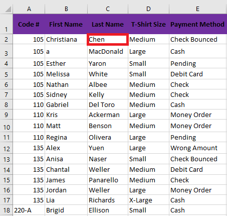
Sorting an Entire Worksheet (Example: by Last Name)
To sort a full dataset alphabetically by a column (e.g., Last Name in Column C):
-
Click a cell in the column you want to sort (e.g., C2).
-
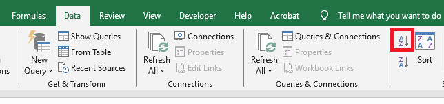
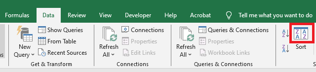
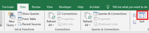
Go to the Data tab and click either A to Z (ascending) or Z to A (descending).
-
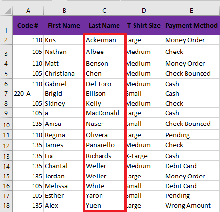
The sheet will be sorted based on the selected column. All rows will adjust accordingly to maintain data integrity.
Sorting a Range Only (Example: by Number of T-Shirts Ordered)
To sort a selected range (e.g., G2:H6) by the number of T-shirts:
-
Highlight the range of cells you want to sort.
-
Click the Sort command in the Data tab.
-
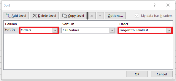
In the Sort dialog box, choose the column to sort by (e.g., « Orders »).
-
Specify the sort order (e.g., Largest to Smallest).
-
Click OK. Only the selected range will be sorted—other parts of the worksheet remain unchanged.

If sorting doesn’t work correctly, double-check for typing errors or inconsistent data formats (e.g., text vs. numbers).
Custom Sorting (Using a Custom List)
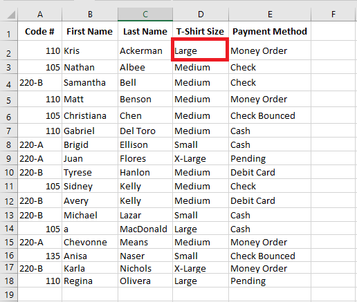
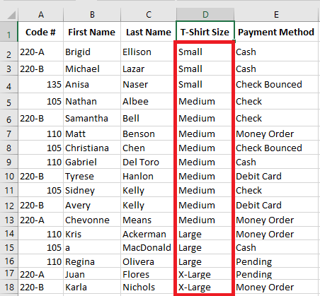
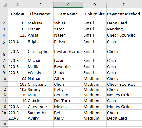
Default sorting in Excel (alphabetical or numerical) may not always suit your needs. When sorting items like T-shirt sizes (Small, Medium, Large, X-Large), alphabetical sorting is inappropriate. Here’s how to apply a custom sort order:
-
Select a cell in the target column (e.g., D2 for T-shirt sizes).
-
Click Sort in the Data tab.
-
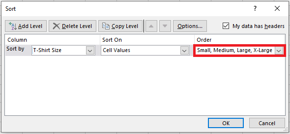
In the Sort dialog, choose the relevant column, then under “Order”, click Custom List.
-
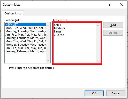
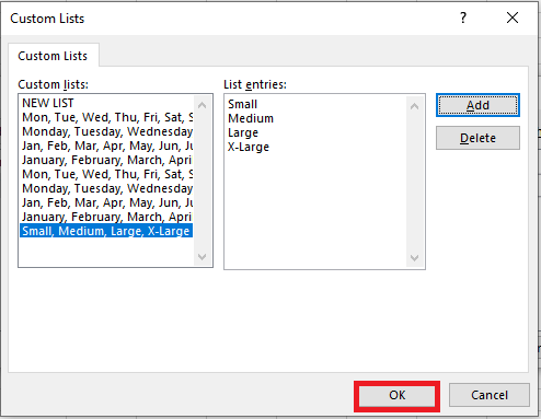
In the Custom Lists window, select New List and type your custom sequence (e.g., Small, Medium, Large, X-Large), pressing Enter after each entry.
-
Click Add then OK to apply the sort.
-
Click OK again in the Sort dialog. Your data will now be sorted according to the custom list.
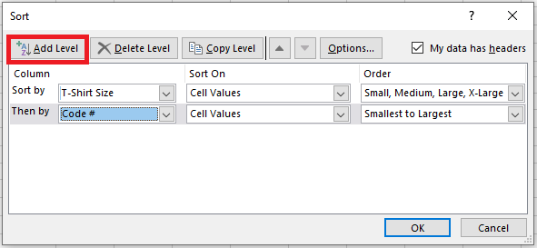
Multi-Level Sorting (Sorting by Multiple Columns)
To gain more control, you can sort data based on multiple criteria (e.g., first by T-shirt size, then by order code):
-
Select any cell in your dataset.
-
Click Sort on the Data tab.
-
In the Sort dialog:
-
Set the first level (e.g., « T-shirt Size ») and choose the custom list as the order.
-
Click Add Level, then define the second level (e.g., « Order Code »).
-
-
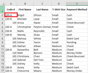
Click OK to apply. Excel will first group data by size, then within each group, sort by code.
Sorting Horizontally (By Rows Instead of Columns)
Although most Excel sorts are vertical (by columns), you can also sort horizontally—i.e., rearranging columns based on values in a particular row. This is useful in non-traditional layouts like side-by-side comparisons.
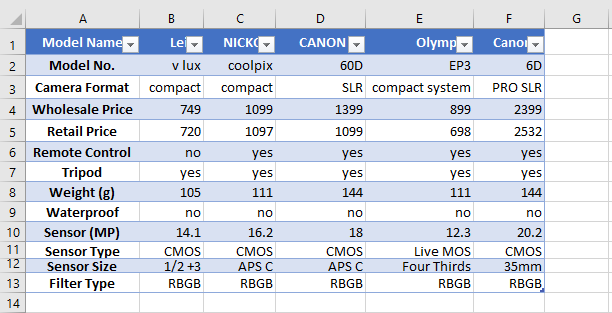
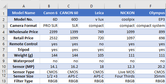
Example: You want to sort camera models based on their names (row 1) or prices (row 4):
-
Select the data range (e.g., B1 to F5). Avoid selecting the first column (A) if it contains feature labels.

-
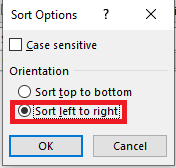
Go to Data > Sort, then click Options in the Sort dialog.

-
In Sort Options, choose Sort left to right, then click OK.
-
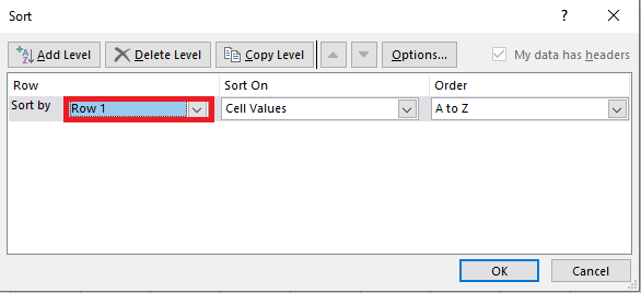
Back in the main Sort dialog:
-
Under “Sort by,” select the row to use (e.g., Row 1 for model names or Row 4 for prices).
-
Choose sort order (A to Z or Smallest to Largest).
-
-
Click OK. Excel will rearrange entire columns based on the selected row’s values.
Excel preserves data integrity by moving full columns rather than individual cells.
Note: This horizontal sorting method can be used to sort by any critical parameter—image sensor size, camera weight, resolution, etc.—depending on your specific need.
-
Filtering Records in Excel
When your spreadsheet contains a large amount of data, it can become challenging to quickly locate the information you need. Excel’s filtering feature allows you to refine your data view by displaying only the rows that meet specific criteria. Below is a comprehensive guide to using filters effectively in Excel.
Applying Basic Filters
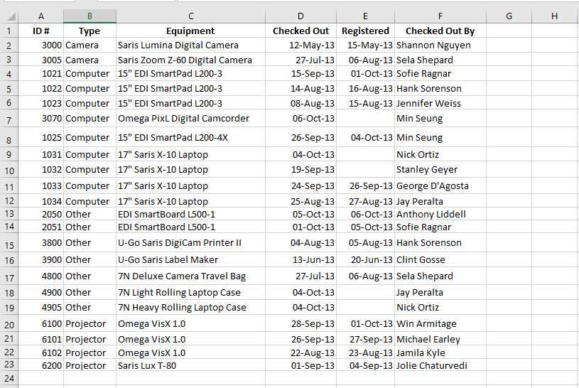
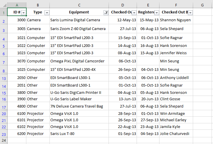
In this section, we’ll apply a filter to an equipment log spreadsheet to display only laptops and projectors that are available for payment.
-
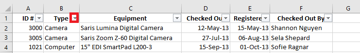
Ensure your spreadsheet has a header row. This row (usually the first) contains labels for each column such as ID#, Type, Equipment, etc. These labels are required for Excel to identify which fields to filter.
-
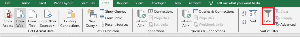
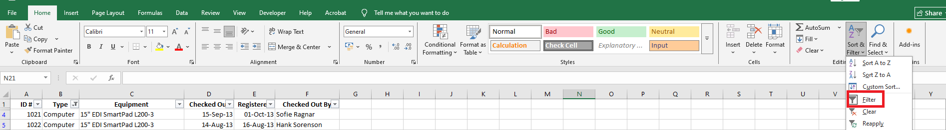
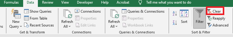
Go to the Data tab and click the Filter command.
-
A dropdown arrow will appear next to each header cell.
-
Click the dropdown arrow in the column you wish to filter. For instance, filter Column B to display only specific equipment types.
-
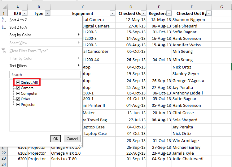
The filter menu will appear.
-
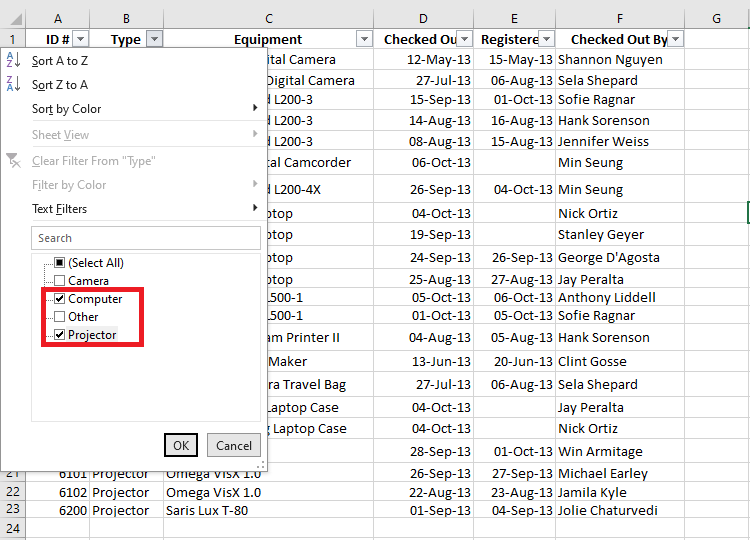
Uncheck “Select All” to quickly deselect everything.
-
Then, check only the options you wish to display — in this example, “Laptop” and “Projector”. Click OK.
-
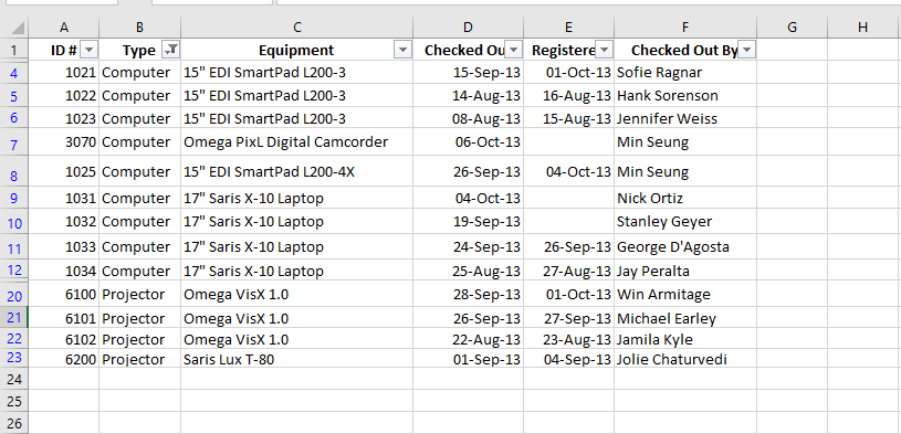
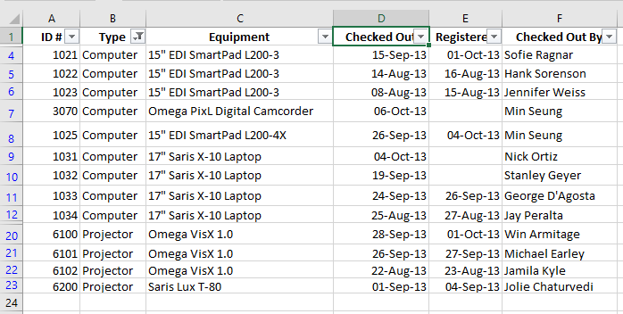
Excel will now hide all rows that do not match the selected values, making only laptops and projectors visible.
You can also access filtering options via the Home tab under the “Sort & Filter” group.
Applying Multiple Filters
Excel allows cumulative filtering, meaning you can apply multiple filters across different columns to narrow down results even further.
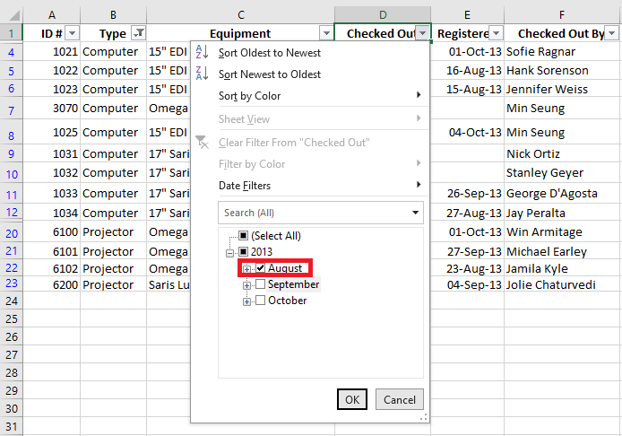
Let’s say the sheet is already filtered to show only laptops and projectors, and now you want to display only those items that were checked out in August:
-
Click the dropdown arrow in the Date column (e.g., Column D).
-
The filter menu appears.
-
Deselect all other months except August, then click OK.
-
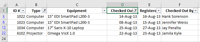
Your spreadsheet will now show only laptops and projectors that were checked out in August.
Clearing Filters
Once you’re done analyzing, you may want to remove filters:
-
Click the dropdown arrow of the filtered column (e.g., Column D).
-
Choose Clear Filter From [Column Name].

-
All previously hidden rows will reappear.
To remove all filters in one click, go to the Data tab, click on the Filter command, and then choose Clear.
Using Advanced Filtering Options
If basic filters aren’t sufficient, Excel provides advanced filtering tools like search, text filters, date filters, and number filters to help pinpoint specific data.
Filtering with the Search Box
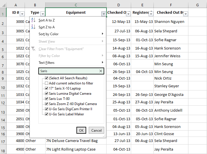
Let’s say you want to view only equipment from the brand “Saris”:
-
Click the dropdown arrow in the Brand column (e.g., Column C).
-
In the search box, type Saris.
-
Excel will dynamically display matching options. Select them and click OK.
-
The sheet will now show only rows containing the brand “Saris”.
Using Advanced Text Filters
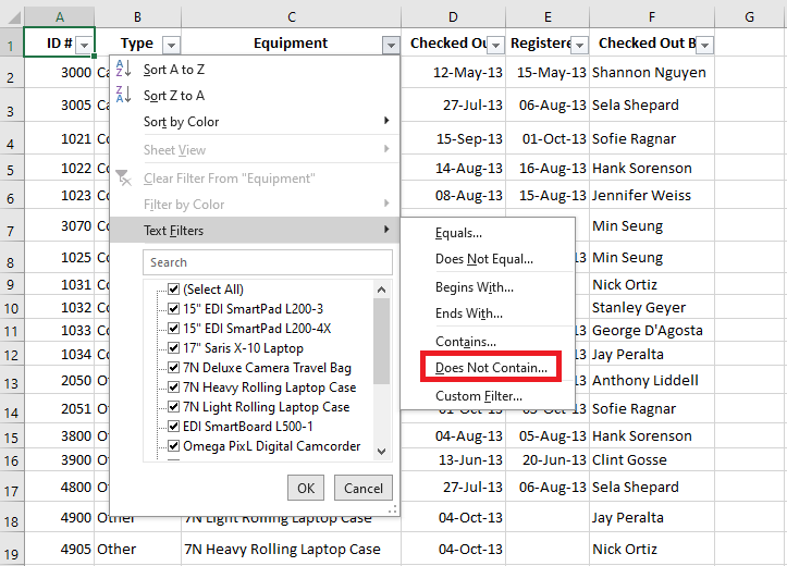
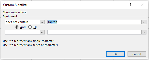
Text filters allow for even more control. For example, to exclude all items containing the word Laptop:
-
Click the dropdown arrow in Column C.
-
Hover over Text Filters and select Does Not Contain…
-
In the dialog box, type Laptop and click OK.
-
The filtered view will now exclude any item that contains the word “Laptop”.
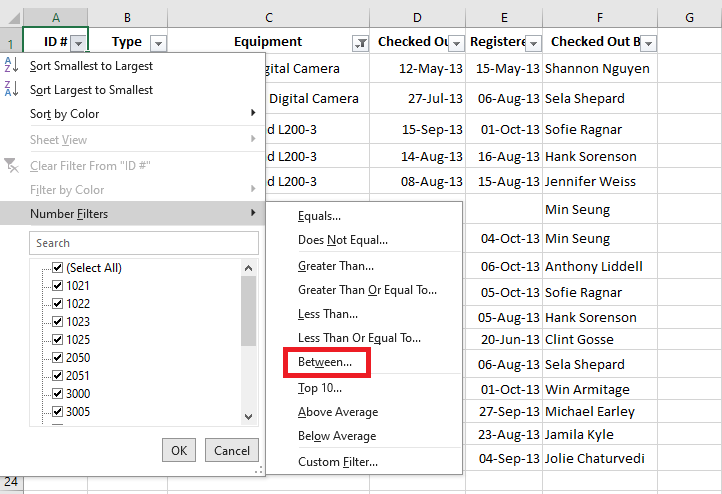
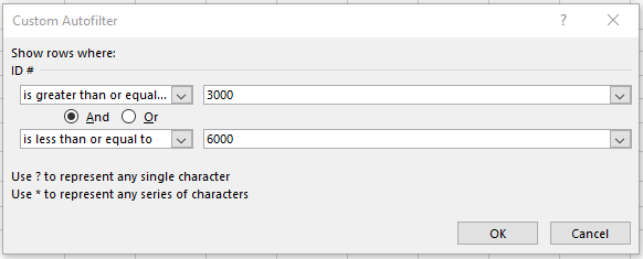
Using Advanced Number Filters
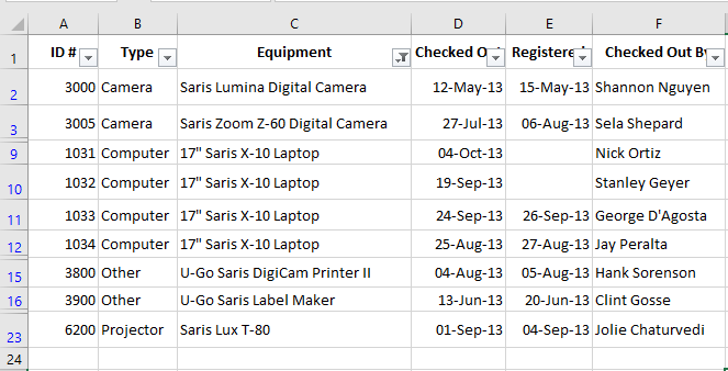
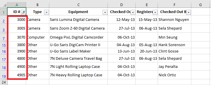
To display equipment with ID numbers between 3000 and 6000:
-
Click the dropdown in the ID# column (A).
-
Hover over Number Filters, and choose Between…
-
Enter 3000 and 6000, then click OK.
-
Excel will now display only items with IDs in the specified range.
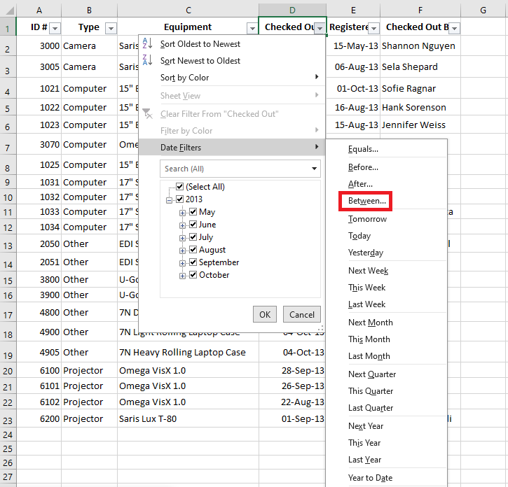
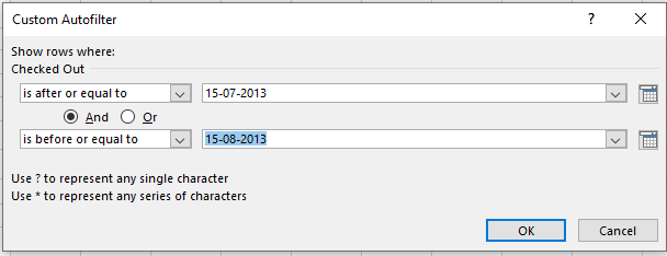
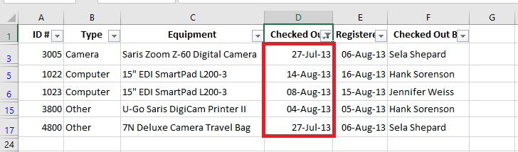
Using Advanced Date Filters
To filter equipment retrieved between July 15 and August 15:
-
Click the dropdown arrow in the Date column (D).
-
Hover over Date Filters, and choose Between…
-
Enter 15-07-2013 and 15-08-2013 (or in your local format), then click OK.
-
The spreadsheet will display only items retrieved within this date range.
These filtering techniques are powerful tools for managing large datasets efficiently in Excel. Whether you’re dealing with text, numbers, or dates, filters allow you to quickly extract meaningful insights from your data.
-
Inserting Total Rows in Excel Tables
Adding a Total Row to Your Excel Table
Once your dataset has been converted into an Excel Table, adding a Total Row becomes a simple and powerful feature that enhances your data analysis. There are two main methods to add a Total Row:
Method 1: Using the Ribbon
-
Click anywhere inside your Excel Table.
-
Go to the Table Design tab on the Ribbon (also called Design in some versions).
-
In the Table Style Options group, check the box labeled Total Row.
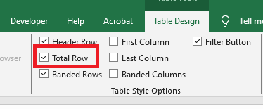
You will now see a new row added at the bottom of your table, displaying the total for the last column by default.
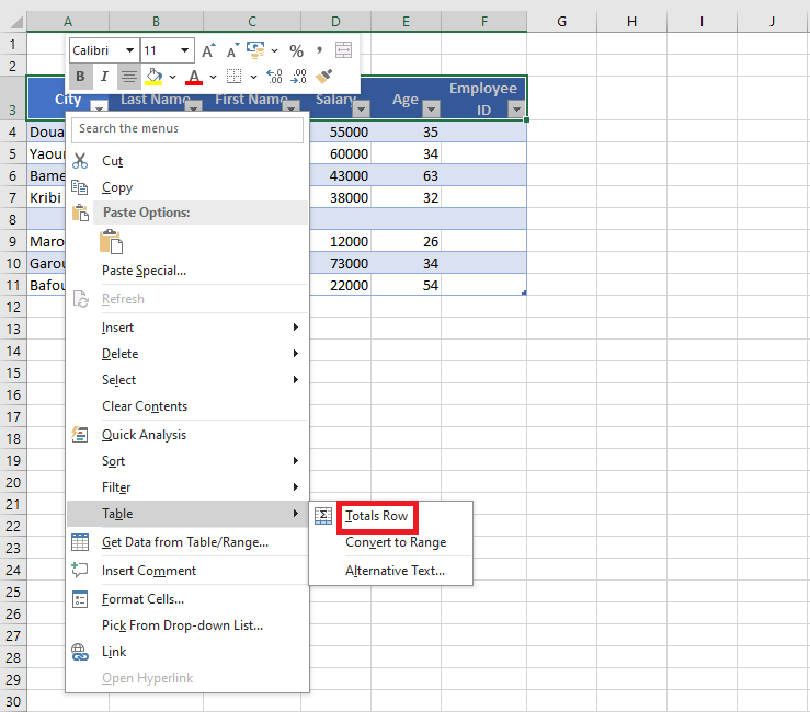
Method 2: Using the Right-Click Menu
-
Right-click any cell within your Excel Table.
-
Hover over Table in the context menu.
-
Click Total Row from the submenu.
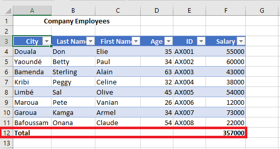
Whichever method you use, Excel will insert a Total Row at the bottom of the table. By default, it will apply the SUM function to the last column, but this can easily be changed.
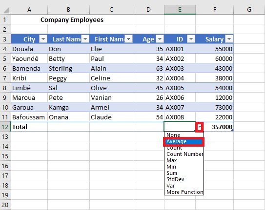
Once the Total Row appears, you can customize each cell in that row. Simply click any cell in the Total Row and a drop-down arrow will appear. This drop-down gives you a variety of aggregation functions to choose from.
Using Other Aggregation Functions in the Total Row
The Total Row is not limited to just sums. It can also display other summary statistics such as:
-
Average
-
Minimum (Min)
-
Maximum (Max)
-
Count
-
Standard Deviation
-
Or even a custom formula of your choice.
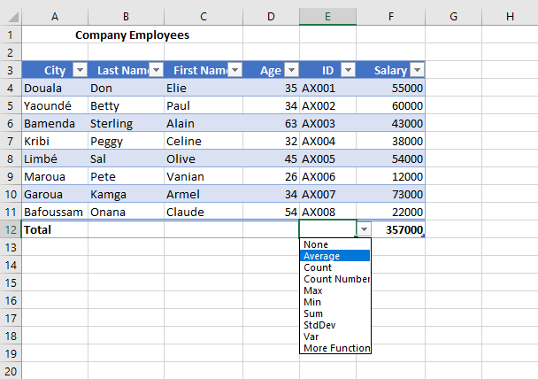
For example, if you want to display the average age from an « Age » column:
-
Click the cell in the Total Row that corresponds to the Age column.
-
Click the drop-down arrow that appears.
-
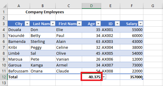
Choose Average from the list.
The cell will now display the average of all values in the Age column.
Most of these calculations use the
SUBTOTALfunction, which you can observe in the formula bar. The advantage of usingSUBTOTALis that it automatically adjusts when you filter your table — it calculates only the visible (filtered) values.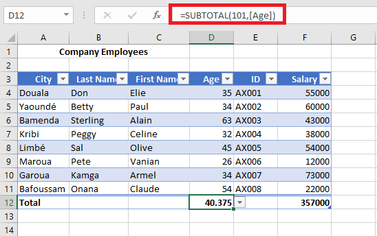
If the predefined list does not offer the function you need, you can insert a different one manually:
-
Click the cell in the Total Row for the desired column.
-
Click the drop-down arrow.
-
Select More Functions at the bottom of the list.
- The Insert Function dialog box will appear, allowing you to choose from any Excel function.
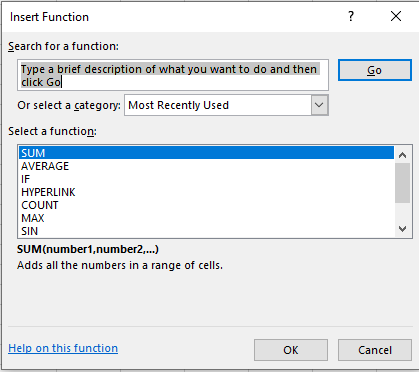
This flexibility allows you to perform customized summaries directly within your table, making the Total Row a valuable tool for quick insights.
-
How to Remove Table Formatting in Excel
By default, Excel tables come with a wide range of built-in features, including predefined table styles that enhance readability and presentation. However, in certain scenarios, you may want to remove the table’s formatting while preserving its structure and functionality.
Remove Table Style Formatting Only
If your goal is to remove the default table style but keep the benefits of a functional Excel table (such as automatic expansion, structured references, and filter buttons), follow these steps:
-
Click on any cell within the table.
-
Go to the Table Design tab (or Design tab under older versions).
-
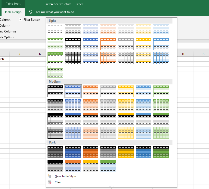
In the Table Styles group, click the very first style under the Light category, labeled None.
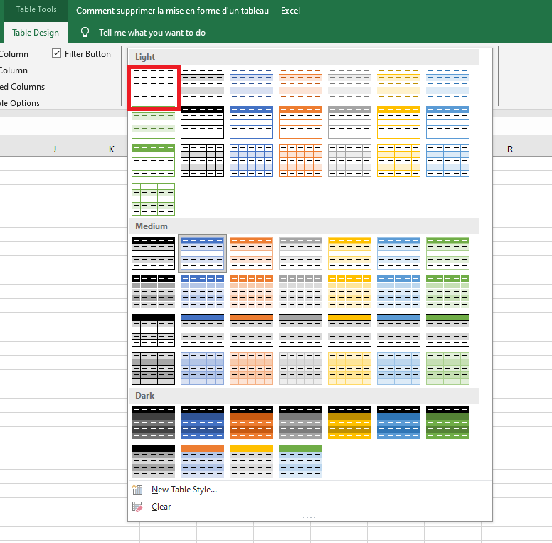
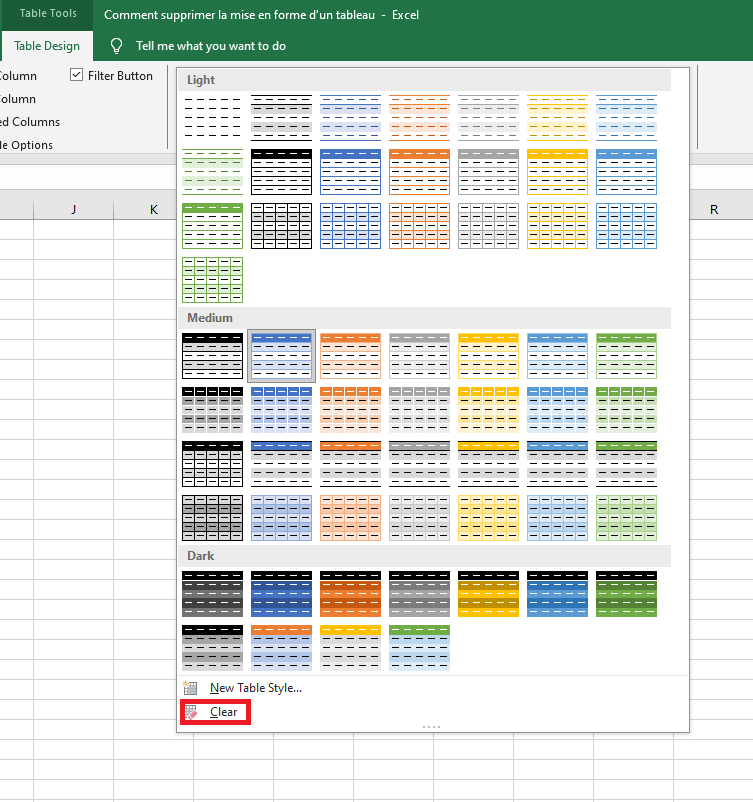
- Alternatively, click the dropdown arrow (the « More » button) in the Table Styles gallery, then click Clear at the bottom of the list.
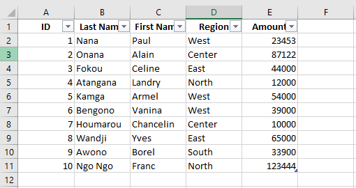
This will strip away the applied style, but your data will remain in a fully functional Excel table — just without the visual enhancements.
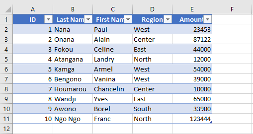
BEFORE
AFTER
-
These options only remove the built-in style formatting. Any custom formatting (such as fonts, colors, borders, etc.) that was manually applied will remain.
-
This method is especially useful when you want to leverage Excel table features but retain your existing cell formatting. Simply convert your data to a table, then clear the style to preserve your custom appearance.
-
To apply a new look, you can always choose another style from the table style gallery.
Clear All Formatting from a Table
If some formatting remains after clearing the table style — such as custom fills, fonts, or borders — it means that manual formatting was applied. To completely remove all formatting (both predefined and custom), do the following:
-
Click on any cell in the table.
-
Press Ctrl + A twice to select the entire table, including headers.
-
Navigate to the Home tab.
-
In the Editing group, click Clear → Clear Formats.

This action will remove all forms of formatting, including:
-
Table styles
-
Manually applied cell formatting
-
Number formats
-
Text alignment
-
Font colors and fills
Caution: This method will reset all formatting. Ensure you’re okay with losing number formats, alignments, and any other styling before proceeding.
BEFORE
AFTER
-
How to Customize and Apply Table Styles in Excel
Creating and managing custom table styles in Excel allows you to define consistent formatting that aligns with your personal or organizational preferences. Follow the detailed steps below to create, edit, apply, or remove a custom table style.
Creating a Custom Table Style
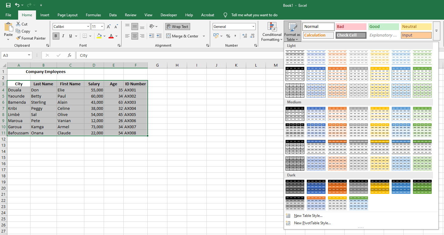
-
Navigate to the Home tab on the Ribbon and click Format as Table.
-
At the bottom of the style gallery, click New Table Style to open the customization window.

-
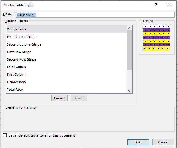
In the New Table Quick Style dialog box, you can assign a custom name to your new style. For this example, we will retain the default name.
-
From the Table Element list, select the component you wish to format first — for instance, Header Row.
-
Click the Format button to open the cell formatting dialog.

-
In the Format Cells window, apply the desired formatting options. For example, you can set a specific background color, font style, or border for the header row.
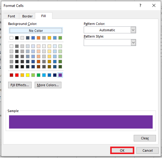
-
Once you’re done with the formatting for that element, click OK to return to the style editor.
-
Repeat the process for other elements in the Table Element list, such as banded rows, total row, or first/last column.
-
As you make changes, a Preview box shows how your table will look with the applied formatting.
- Optionally, you can adjust the stripe size for banded rows or columns. This determines how many rows or columns each stripe covers.

-
At the bottom, you’ll find a checkbox labeled Set as default table style for this document. Select this if you want all new tables in this workbook to use your custom style by default.
-
When finished, click OK to save the new style.
Your custom table style is now created and available for use in the current workbook.
Applying a Custom Table Style
-
Select any cell within the range you wish to convert into a table.
-
Click Format as Table in the Home tab toolbar.
-
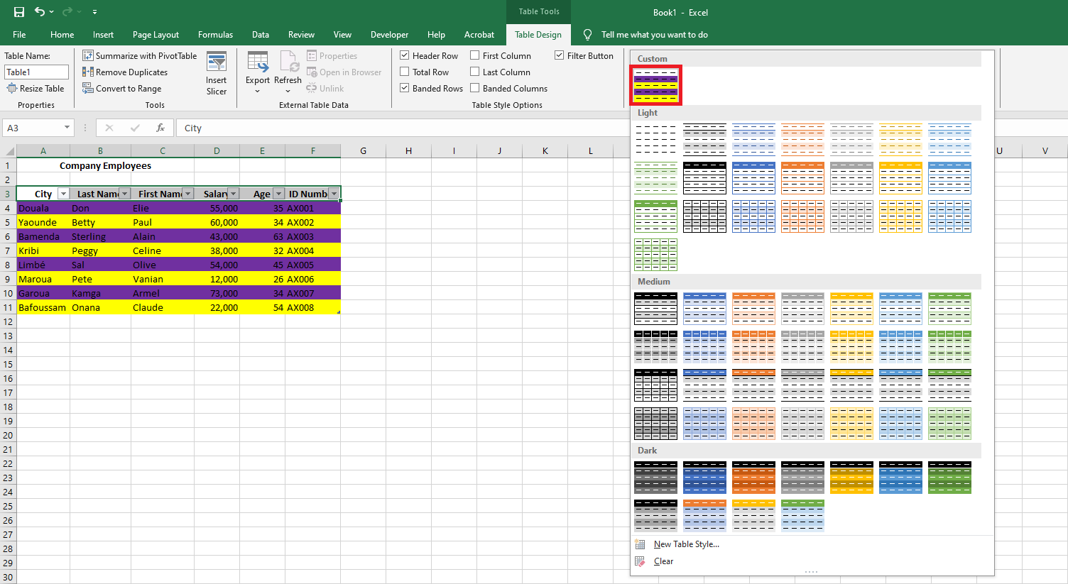
Scroll through the style gallery to locate your newly created style.
-
Hover over the style to preview how it would look on your table.
-
Click on the style to apply it.
Note: Custom table styles are workbook-specific. They will not be available in other Excel files unless redefined.
Modifying a Custom Table Style
-
Go to the Format as Table menu in the Ribbon.
-
Right-click on the custom style you wish to change.
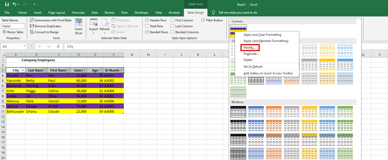
- From the context menu, select Modify. This reopens the style editor where you can change the formatting settings.
- Alternatively, if you want to create a slightly different version while keeping the original intact, choose Duplicate instead.
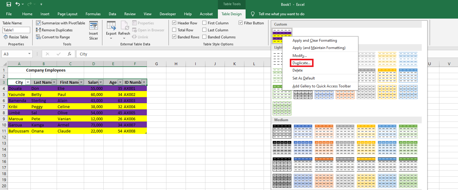
- Excel will append “2” to the name of the duplicated style, which you can rename as needed.

-
Click OK once you’ve finalized the changes. Now, both the original and duplicated styles will appear in the gallery.

Deleting a Custom Table Style
If a custom style is no longer needed and hasn’t been applied to any tables, you can remove it to free up memory.
-
Open the Format as Table menu.
-
Right-click the style you want to remove.
- Select Delete from the context menu.

-
Confirm the deletion by clicking OK when prompted.

If any tables currently use the deleted style, Excel will revert them to the default formatting.
-
Applying Styles to Excel Tables
Once you’ve created a table in Excel, the first thing you’ll likely want to do is make it visually appealing and easy to interpret. Thankfully, Microsoft Excel offers a wide array of built-in table styles that allow you to instantly format or reformat a table with just one click. And if none of the default styles meet your specific design preferences, you can quickly define your own custom style.
Moreover, Excel allows you to toggle key table elements on or off — such as the header row, banded rows, total row, and more — giving you full control over the appearance and behavior of your table.
Built-in Table Styles
Excel tables are designed not just for data storage but for enhanced data management. They offer features like built-in filtering and sorting, calculated columns, structured references, and automatic total rows. When you convert a regular data range into a table, Excel automatically applies default formatting: alternating row colors (banded rows), border lines, and font styling.
If you’re not satisfied with the default format, you can easily change it via the Design tab that appears under Table Tools when a cell in the table is selected.
Example: Over 50 Built-in Table Styles
As shown in the illustration (Fig. 3.2.1.a), Excel provides a gallery of over 50 pre-defined styles, categorized as Light, Medium, and Dark themes. A table style acts as a formatting template, automatically applying visual elements to headers, rows, columns, and the total row.
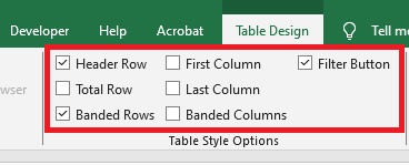
You can further customize your table using the Table Style Options, which allow you to control the appearance of specific elements:
-
Header Row – Show or hide the table headers.
-
Total Row – Add a summary row at the bottom of the table, with built-in functions for each column.
-
Banded Rows / Columns – Alternate shading for improved readability.
-
First/Last Column – Apply special formatting to highlight these columns.
-
Filter Button – Show or hide the dropdown filter arrows in the header row.
Choosing a Table Style While Creating a Table
To create a table and immediately apply a specific style, follow these steps:
-
Select the cell range you want to convert into a table.
-
On the Home tab, go to the Styles group, and click Format as Table.
-
In the style gallery, click the table style you want to use.
Changing the Style of an Existing Table
To change the appearance of a table that already exists:
-
Click any cell inside the table.
-
Go to the Design tab under Table Tools, and in the Table Styles group, click the More arrow to see all available styles.
-
Hover over a style to preview it live on your table. Click to apply it.
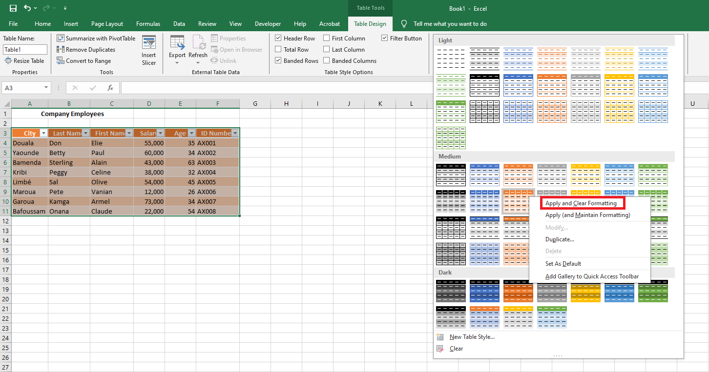
Tip: If you previously applied custom formatting (like bold fonts or custom colors) manually to some cells, Excel will retain them even when you switch styles. To override this and apply the new style completely, right-click the style and choose Apply and Clear Formatting.
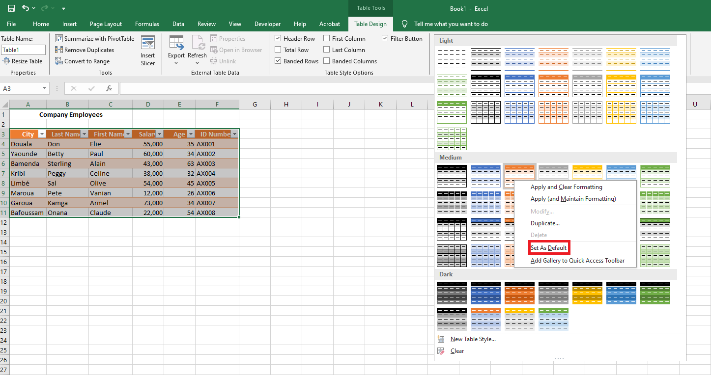
5.4 Setting a Default Table Style for a Workbook
If you want every new table in your workbook to follow a specific style, set it as the default:
-
In the Table Styles gallery, right-click your preferred style.
-
Select Set As Default.
From now on, every table inserted via the Insert tab will adopt this style automatically.
Applying Table Styles Without Creating an Actual Table
If your goal is to quickly style a data range without converting it into a structured Excel table, here’s a workaround:
-
Select the data range you wish to format.
-
On the Home tab, in the Styles group, click Format as Table, then choose your desired style.
-
After the table is created, go to the Design tab and click Convert to Range to revert it back to a regular range.
-
Structured References in Excel Tables
One of the most powerful and practical features of Excel tables is the use of structured references. At first glance, this special syntax for referencing table data may appear complex or even confusing, especially if you’re accustomed to traditional cell references. However, once you begin to work with it, you’ll quickly discover how useful and efficient this functionality can be—especially in dynamic data environments.
A structured reference, also known as a table reference, is a specific way to refer to parts of an Excel table by using the table’s name and column headers, rather than standard cell addresses like A1 or B2. This makes formulas easier to read, more intuitive, and more resilient to changes.
The reason this type of referencing is so essential lies in the inherent power of Excel tables: unlike regular cell ranges, tables automatically expand or contract when data is added or removed. Standard cell references do not adapt to these changes, which can lead to inaccurate results or broken formulas. Structured references, on the other hand, dynamically adjust to include new rows or columns, ensuring that your formulas always remain up to date.
For instance, to sum the values from cells B2 to B5 using a regular cell range, you would write:
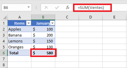
=SUM(B2:B5)But if your data is organized in an Excel table named SalesTable, and you want to sum the values in the « Sales » column, you would use a structured reference like this:
=SUM(SalesTable[Sales])This formula is not only easier to interpret (you know exactly what it sums), but it will also automatically include any new sales data added to the table.
Key Features of Structured References in Excel
Compared to standard cell references, structured references offer several advanced features that enhance both the flexibility and efficiency of working with data in Excel tables:
■ Easy to Create
Structured references are incredibly simple to insert into a formula. You don’t need to memorize any special syntax—just select the desired table cells with your mouse, and Excel automatically generates the correct structured reference. This makes it accessible even to users unfamiliar with the syntax.■ Automatically Resilient and Self-Updating
One of the greatest advantages of structured references is their ability to automatically adapt to changes. When you rename a column in a table, all associated structured references are immediately updated to reflect the new column name—eliminating the risk of broken formulas. Furthermore, when you add new rows to the table, those rows are seamlessly included in existing references, ensuring that formulas always cover the entire data range.This means that no matter how frequently your data changes, your structured references remain accurate and up to date, reducing the need for manual adjustments.
■ Usable Both Inside and Outside the Table
Structured references are not limited to formulas within the table itself. You can also use them in formulas located outside the table, which is especially helpful in large workbooks where you may need to reference specific tables from various sheets. This improves clarity and makes it easier to manage complex spreadsheets.■ Auto-Fill for Calculated Columns
When you enter a formula in a single cell of a table column, Excel automatically fills the rest of the column with the same formula—creating what’s known as a calculated column. This feature ensures consistency in your computations and saves time by applying the formula to all rows without manual copying.How to Create a Structured Reference in Excel
Creating a structured reference in Excel is both straightforward and intuitive. If you’re starting with a regular range of data, your first step should be to convert that range into an official Excel table. This unlocks all the advanced features of table management, including structured references.
To convert a standard data range into a table:
-
Select the entire dataset.
-
Press Ctrl + T (or Ctrl + L in some older versions of Excel).
-
Make sure the « My table has headers » option is checked, then click OK.
Once your data is formatted as an Excel table, you can create structured references by following these simple steps:
- Begin writing your formula
Start as usual by typing the equals sign (=) in the desired cell. - Select the relevant cells in the table
Instead of typing cell addresses, simply use your mouse to select the cell or range you want to include from within the table. Excel will automatically insert the structured reference using the table name and column headers. This eliminates the need to know the syntax by heart. - Close the formula and press Enter
Once your structured reference is inserted, complete the formula by typing the closing parenthesis)and pressing Enter. If you’re entering the formula inside the table, Excel will automatically fill the entire column with the same formula, creating a calculated column.
Example: Summing Monthly Sales
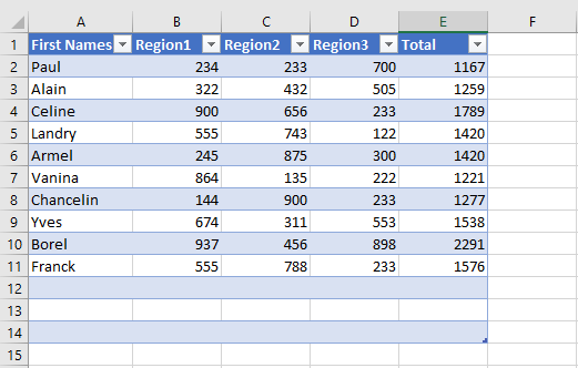
Suppose you have a table namedMonthlySales, and it contains sales figures for three months across columns B, C, and D. You want to calculate the total sales per row in column E.To do this:
-
Click in cell E2 (the first row of your total column).
-
Type:
=SUM( -
Select the cells B2 to D2 (Excel will translate this into a structured reference like =SUM(Article[@[January]:[March]]) depending on your column headers).
-
Type the closing parenthesis
)and press Enter.
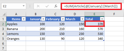
As a result, the entire column E is automatically filled with the following formula:
=SUM(MonthlySales[@[January]:[March]])Even though the formula looks identical across all rows, Excel evaluates it individually for each row using the respective data. This row-wise behavior is one of the most powerful aspects of structured references in Excel tables.
Creating Structured References Outside of a Table
If you’re entering a formula outside of the table and only need to refer to a specific column or range of data within the table, you can quickly create a structured reference without manually selecting the cells. Here’s how:
- Begin typing the formula normally.
For example, to calculate the maximum value in a column, you might start typing=MAX(. - Type the first few letters of the table name.
As soon as you type the first letter, Excel will display a dropdown list of all table names that match what you’re typing. The more letters you type, the more refined the list becomes. - Use the arrow keys to select the correct table.
Scroll through the list using the up/down arrow keys on your keyboard. - Press Tab or double-click to insert the table name.
Once the correct table is selected, press Tab or double-click the name to insert it into your formula. - Complete the formula and press Enter.
Add any column reference or closing parentheses needed and press Enter.
Example:
Let’s say you want to find the highest value in a table named Article.-
You begin by typing
=MAX( -
Then type “Ar”
-
Excel shows Article as a suggestion
-
Press Tab to select it
-
Complete the formula with
)and hit Enter
Your final formula looks like this:
=MAX(Article)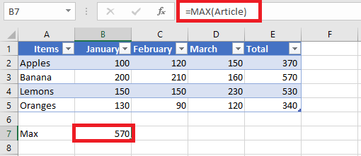
Structured Reference Syntax in Excel
As previously mentioned, you don’t necessarily need to master the syntax of structured references to use them in formulas—Excel inserts them automatically as you work with tables. However, understanding this syntax will help you interpret what your formulas are actually doing, especially when analyzing or debugging them.
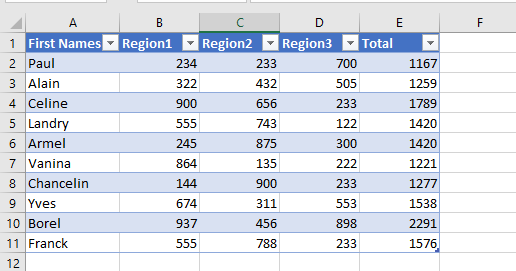
In general, a structured reference is a text string that starts with the table name and ends with one or more column specifiers. To illustrate, let’s break down the following formula which adds the values from the “South” and “North” columns in a table named Regions:
This structured reference contains three main components:
-
Table name
-
Item specifier
-
Column specifier(s)
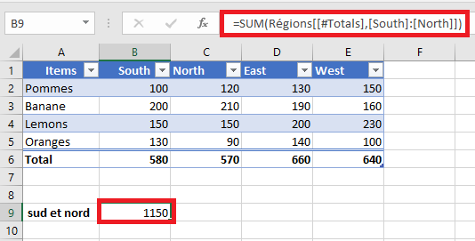
When you select the cell containing this formula and click into the formula bar, Excel highlights the exact cells involved in the calculation, helping you visualize the data being referenced.
Table Name
The table name refers only to the data body of the table—it excludes both the header row and the total row. This name may be the default (e.g.,
Table1) or a custom name likeRegions.
If your formula is located inside the same table, Excel often omits the table name because it is implicitly understood.Column Specifier
A column specifier refers to the data within a specific column, excluding the header and total rows. It is written inside square brackets.
For example:To reference multiple adjacent columns, you can use a range operator (colon), like this:
If a column name contains spaces, punctuation, or special characters, Excel adds an extra set of square brackets:
Item Specifier
To reference specific parts of a table (such as the entire table or just the headers), Excel uses item specifiers. These always begin with a hash symbol (
#) except for row-specific references using@.Item Specifier Description [#All]Refers to the entire table (data, headers, and totals) [#Data]Refers only to the data rows [#Headers]Refers to the column headers [#Totals]Refers to the total row (returns null if the total row is not visible) [@ColumnName]Refers to the same row as the formula, within the specified column For example, to sum values from the South and West columns in the current row, you would write:Structured Reference Operators
Structured references support various operators that enhance their flexibility:
• Range Operator (
:)Used to reference a range of adjacent columns. For example:
This sums the current row’s values from “South” to “West”.
• Union Operator (
,comma)Used to reference non-adjacent columns. For instance:
This adds values from the “South” and “West” columns in the same row.
• Intersection Operator (
Used to refer to the value at the intersection of a specific row and column. For example, to return the value at the intersection of the Total row and the West column:
Note: In this case, the
[#All]specifier (or a similar item specifier) is essential, because column specifiers alone do not include the total row. Without it, Excel may return a#NULL!error.Syntax Rules for Structured Table References
When manually editing or creating structured references in Excel tables, it’s important to follow specific syntax rules to ensure formulas work properly and remain readable. Below are the main guidelines to follow:
Enclose Specifiers in Brackets
All column specifiers and special item identifiers must be enclosed in square brackets[ ]. If a specifier includes multiple elements or a range, it should be wrapped in an additional set of brackets.
Example:
To reference a range from the “South” column to the “West” column in the current row:=Regions[@[South]:[West]]Separate Multiple Specifiers with Commas or Semicolons
When combining two or more inner specifiers within a single reference, separate them with commas (,in English versions) or semicolons (;in French versions), depending on your regional Excel settings.
Example:
To reference the column header for « South » within a structured reference, use an additional set of brackets and separate specifiers:=Regions[[#Headers],[South]]Do Not Use Quotation Marks Around Column Headers
In structured references, column headers should not be enclosed in double quotes—even if they contain text, numbers, or dates. Excel automatically interprets them based on the table’s metadata.Use Single Quotes for Special Characters in Column Headers
Certain characters within column headers—such as square brackets[ ], the pound/hash symbol#, and the single quote'—have special meaning in Excel. If one of these appears in a column name, precede it with a single quote (') within the reference to avoid syntax errors.
Example:
If a column is namedItem #, you must escape the#with a single quote:=Regions[[#Headers],[Item '#]]Use Spaces to Improve Readability
While not mandatory, inserting spaces between specifiers (especially after commas or semicolons) improves the clarity and readability of complex structured references.
Example:
To average the values in columns “South”, “North”, and “West” from the current row, you can use:=AVERAGE(Regions[@[South]]; Regions[@[North]]; Regions[@[West]])Structured References in Excel Tables
To better understand how structured references work in Excel tables, let’s review a few practical and illustrative examples. These examples are designed to be simple, meaningful, and applicable to real-world scenarios.
Counting Rows and Columns in an Excel Table
To determine the number of columns or rows in a table, you can use the built-in Excel functions
COLUMNSandROWS, which only require the table name as input:These formulas return the total number of columns and data rows in the table named
Sales.If you want to include both the header row and the Total Row (if present), use the special item specifier
[#All]:=ROWS(Sales[#All])This will return the number of all rows including the header and total rows.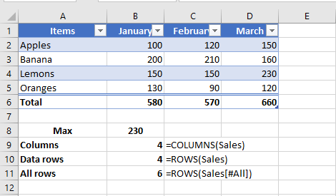
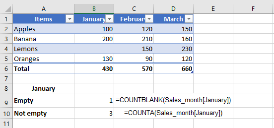
Counting Blank and Non-Blank Cells in a Specific Column
When working with a specific column in a table, you may want to count how many cells are empty or contain data. Be sure to place your formula outside of the table to avoid circular references and incorrect results.
-
To count blank cells:
-
To count non-blank cells:
If your table is filtered and you want to count only the non-blank cells in the visible rows, use the
SUBTOTALfunction with function number103:This version of the formula ignores filtered-out (hidden) rows and only counts visible non-empty cells.
Summing Values in an Excel Table
The fastest way to calculate totals in an Excel table is by enabling the Total Row option:
-
Right-click anywhere inside the table.
-
Select Table from the context menu.
-
Click Total Row.
Excel will add a summary row at the bottom of the table. By default, it may only calculate the total for the last column, leaving the rest empty.
To fix this, click any empty cell in the Total Row, click the dropdown arrow that appears, and choose the SUM function. Excel will insert a structured
SUBTOTALformula that adds only the values from visible rows, ignoring any filtered-out data:Likewise, a regular
SUMfunction using a structured reference (e.g.,=SUM(Sales[January])) won’t work inside the table for the same reason.Relative and Absolute Structured References in Excel
By default, structured references in Excel tables behave according to specific rules, which can impact how formulas respond when copied or dragged across cells:
-
References to multiple columns are absolute by nature. They do not change when the formula is copied or moved across the worksheet.
-
References to a single column are relative when formulas are dragged horizontally across columns, meaning the column reference will adjust. However, when such formulas are copied and pasted using standard commands (Ctrl+C and Ctrl+V), the references remain fixed.
This behavior presents a challenge when you need a combination of relative and absolute references in your table formulas. Dragging a formula will shift single-column references (which may be undesired), while copying and pasting will fix all references (removing the intended dynamic behavior). Fortunately, there are practical tricks to control this behavior precisely.
Absolute Structured Reference to a Single Column
To force a single-column reference to behave like an absolute reference, repeat the column name to explicitly define it as a range.
-
Relative column reference (default):
TableName[Column] -
Absolute column reference:
TableName[[Column]:[Column]]
To refer to the current row with an absolute column reference, use the
@symbol before the column name:-
TableName[@[Column]:[Column]]
Example Use Case
Imagine you want to sum the monthly sales of a specific product over three months. You enter the product name in cell
F2, and use theSUMIFfunction to calculate the total sales for January:However, if you drag this formula to the right to calculate totals for February and March, the
[Items]reference might shift, breaking the formula.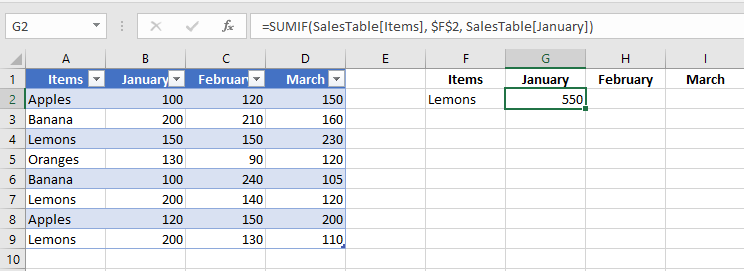
To prevent this, make the
[Items]reference absolute while keeping[January]relative:=SUMIF(SalesTable[[Items]:[Items]], $F$2, SalesTable[January])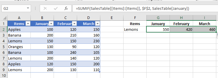 Now, when you drag the formula to adjacent columns, only the third argument (
SalesTable[January]) updates accordingly (to February, March, etc.), while the[Items]column remains fixed.Relative Structured References to Multiple Columns
By default, multi-column structured references in Excel tables are absolute and do not change when copied across cells. This default behavior is generally consistent and expected.
However, if you want to create a relative multi-column structured reference, you can do so by prefixing each column with the table name and removing the outer brackets.
-
Absolute range reference (default):
TableName[[Column1]:[Column2]] -
Relative range reference:
TableName[Column1]:TableName[Column2]
To reference multiple columns in the current row, use the
@symbol with each column:-
@[Column1]:[Column2]
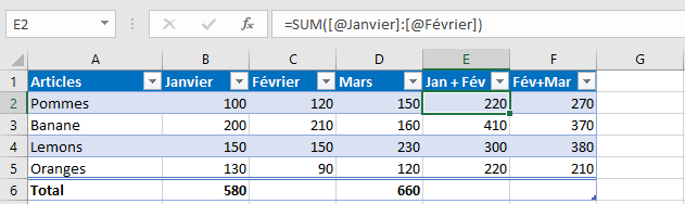
Example: Row-Level Summation
To sum the values in the current row for columns January and February, use:
This reference is absolute, so copying it to another column will still sum January and February.
If you want the referenced columns to adjust relative to the formula’s position, use a relative structured reference like this:
=SUM(Table10[@February]:Table10[@March])
Note that if the formula is written inside the same table, the table name (
Table10) is optional and usually omitted by Excel automatically.-
Difference Between a Data List and an Excel Table
A data list in Excel is simply a range of related information organized in rows and columns. However, when that list is formally converted into an Excel Table, it gains powerful built-in features that enhance data management, analysis, and formatting. Below is a detailed comparison highlighting the key differences between a basic data list and an Excel Table:
Feature Data List Excel Table Header Row Headers must be added manually above the data. You can use multiple rows, and the headers don’t need to be unique. Excel automatically creates a single, dedicated header row. Each column header must be unique. You can easily toggle the visibility of the header row via the ribbon. Data Rows Rows are inserted or deleted manually by selecting ranges. Excel does not restrict these actions, which can lead to formatting errors or broken formulas. Rows are managed using table-aware commands. Excel ensures structural integrity by applying changes to entire rows and maintaining consistent formatting and formulas. Total Row Totals must be added manually beneath the list, and formulas for aggregation (SUM, AVERAGE, etc.) must be entered manually. Excel provides an optional Total Row that can be toggled on or off from the ribbon. Aggregation functions are easily applied using dropdown menus in each column. Sorting and Filtering Sorting and filtering are available, but Excel may prompt you to expand your selection if it doesn’t recognize the data range as structured. Sorting and filtering are built into the table structure. Excel inherently understands the table boundaries, eliminating the need to confirm data ranges. Formatting Formatting must be applied manually. When new rows are added, formatting may not automatically carry over. Excel automatically applies consistent formatting, including banded rows and table styles. New data entries inherit the table’s style by default. Formulas Standard cell references (e.g., A2:A10) must be used and managed manually. Copying or editing formulas across rows may introduce inconsistencies. Tables use structured references (e.g., =SUM(Table1[Sales])), which are more intuitive and robust. Excel automatically applies and updates formulas across all relevant rows.Conclusion
Using an Excel Table instead of a simple data list brings numerous benefits, including improved data integrity, easier formatting, automated calculations, and enhanced readability. Tables are especially helpful when working with dynamic datasets, allowing users to focus more on insights and less on manual adjustments.Resizing an Excel Table
Excel tables are dynamic and can easily be resized to include more or fewer rows and columns, depending on the evolving needs of your data. There are three main ways to resize a table:
-
Adding or removing rows and columns
-
Using the « Resize Table » command
-
Dragging the table corner to adjust its range
Adding or Removing Rows and Columns
Even after a table has been created, you can expand or reduce its size by adding or deleting rows or columns. Whether you insert data directly adjacent to the table or within its current range, Excel automatically applies the table’s formatting style.
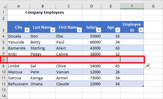
To quickly insert a row or column adjacent to a table:
-
Click in a blank cell next to the table’s current boundary.
-
Enter a value into that cell.
-
Press Enter or click elsewhere to confirm. Excel will automatically include the new cell within the table range and apply the existing formatting.
Note: When you type a formula into an empty column of a table, Excel automatically propagates that formula throughout the column — even for newly inserted rows — without needing to use AutoFill manually.
To insert a row or column using the Ribbon:
-
Select any cell within the table, directly next to where you want to add the new row or column.
Note: You cannot select a column header to use these insertion options. -
Go to the Home tab, click on the Insert drop-down arrow.
-
Choose one of the following options:
-
Insert Table Rows Above – adds a new row above the selected row.
-
Insert Table Columns to the Left – adds a new column to the left of the selected column.
-

To delete unwanted rows or columns from a table:
-
Select a cell within the row or column you want to remove.
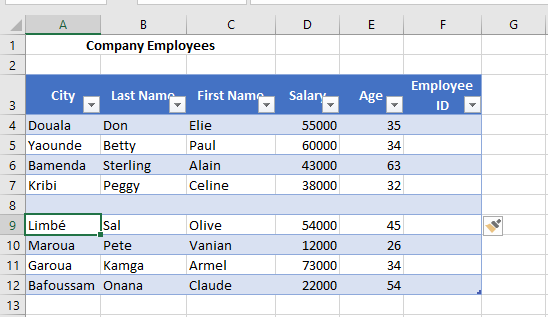
-
Click the Delete drop-down from the Ribbon.
-
Choose:
-
Delete Table Rows
-
Delete Table Columns
-
Resizing a Table Using the « Resize Table » Command
The Resize Table command allows you to explicitly define a new data range for the table. This method is especially useful when you want precise control over the dimensions of the table.
Steps:
-
Click on any cell inside the table.
-
Go to the Table Design tab (visible only when a table cell is selected).
-
Click on Resize Table.
-
In the input field that appears, type the new range you want for the table (e.g.,
A1:E14).

-
Click OK.
The table will be resized accordingly, either expanding or contracting to fit the specified range.
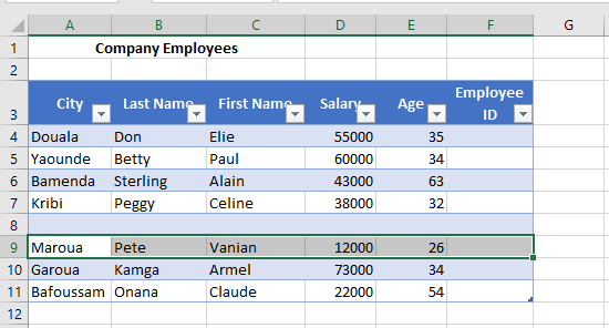
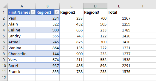
Resizing a Table by Dragging Its Corner
You can also manually resize a table by using the resize handle — a small icon located at the bottom-right corner of the table.
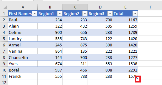
To reduce the table size:
-
Hover over the bottom-right corner of the table until the resize handle appears.
-
Click and drag inward to the desired range, e.g., from
A1:E11toA1:B11.
Note: Cells outside the new table range are no longer part of the table structure, lose their formatting, and no longer participate in formulas referencing the table.
To expand the table size:
-
Hover over the bottom-right corner and click the resize handle.
-
Drag outward to include more rows and/or columns, e.g., from
A1:B11toA1:G11.

The newly added cells are automatically formatted to match the existing table style, and the table’s internal links and formulas extend to include them.
-
Working with Excel Tables and Ranges
Excel tables are among the most powerful features for managing, calculating, and updating structured datasets efficiently. While tables provide enhanced functionality like automatic expansion, structured references, and built-in filters, there may be cases where you need to revert a table back to a regular range—or convert a standard range into a fully functional table.
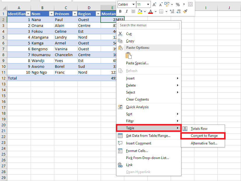
How to Convert an Excel Table to a Normal Range
If you wish to remove table functionality while keeping your data intact, Excel offers a quick way to convert a table into a normal range. Follow these steps:
- Method 1 (Right-click method):
Right-click any cell within the table. From the context menu, select Table > Convert to Range.
- Method 2 (Using the Ribbon):
- Select any cell in the table to activate the Table Design tab.
- On the Table Design tab (formerly « Design » in older versions), locate the Tools group and click Convert to Range.
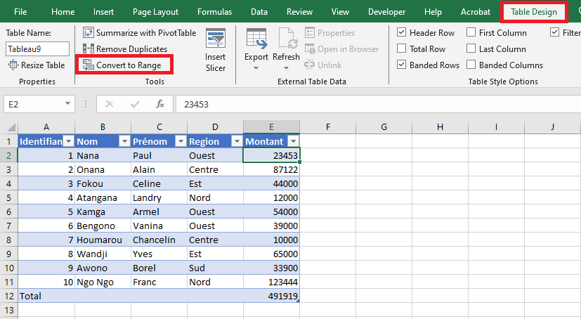
In both cases, Excel will prompt you with a confirmation dialog.
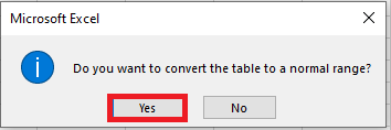
Click Yes to proceed. Once confirmed, the table will be converted to a regular range.
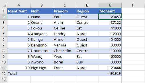
Note that while this process removes table-specific features—such as automatic column expansion, structured formulas, and filter buttons—it preserves the visual formatting (e.g., font colors, cell fill, and borders) applied by the table style.
Converting a Normal Range to an Excel Table
To leverage the full capabilities of Excel tables, you can convert any range of data into a table. There are multiple ways to do this:
- Quick Shortcut Method:
- Select any cell within your data range.
- Press Ctrl + L (or Ctrl + T in newer versions).
-
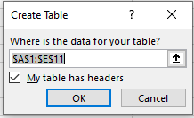
- In the Create Table dialog box, verify the selected range. If your data includes headers, ensure the My table has headers checkbox is selected.
- Click OK.
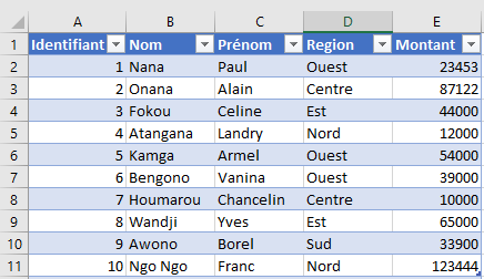
The selected range will instantly become an Excel table, adopting the default table style.
Using the Ribbon to Create a Table
You can also create a table using the ribbon interface:
- Select any cell within your dataset.
- Go to the Insert tab.
- In the Tables group, click Table.
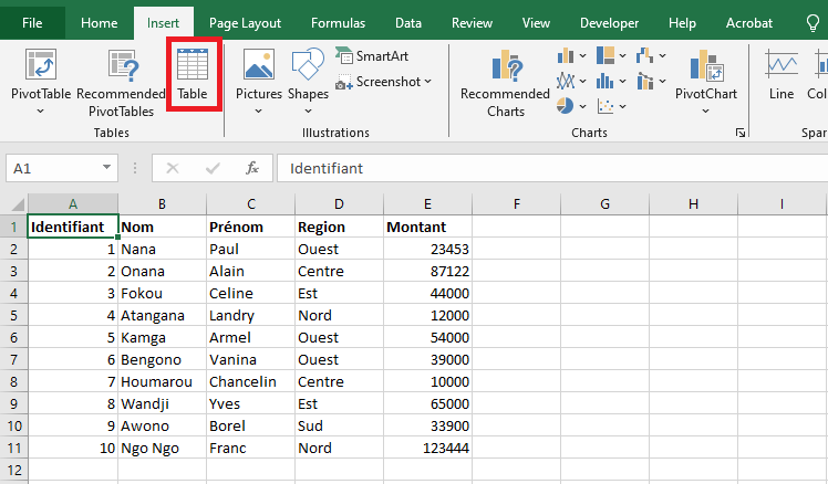
- In the Create Table dialog box, confirm the range and header option, then click OK.
Just like the shortcut method, this action transforms your range into a table with the default style applied.
Converting a Range to a Table with a Specific Style
If you want to apply a specific visual style to your new table right from the beginning, proceed as follows:
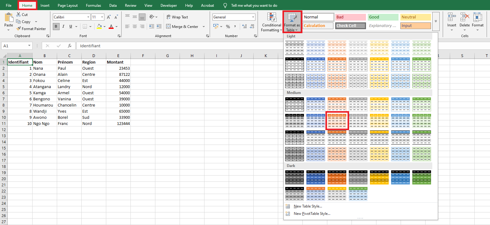
- Select any cell within your dataset.
- Navigate to the Home tab.
- In the Styles group, click Format as Table.
- Choose your preferred table style from the gallery.
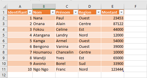
- In the Create Table dialog, confirm the selected range and whether it contains headers, then click OK.
The selected range is now formatted as a table using the chosen style.
If your dataset already has custom formatting and you want to apply the table style without conflicts, you can right-click the style in the gallery and select Apply and Clear Formatting. This option will remove any existing formatting before applying the table style, ensuring consistency and avoiding design clashes.
- Method 1 (Right-click method):