Catégorie : Excel function

This function calculates the Macauley Duration (named after its developer) of a fixed-interest security, representing the weighted average time until all cash flows (interest and principal) are received.

Syntax

DURATION(Settlement; Maturity; Nominal_Interest; Yield; Frequency; [Basis])

Arguments

• Settlement (required)
  The date of purchase for the security. Time values are truncated.
• Maturity (required)
  The maturity date when the principal is repaid. Time values are truncated.
• Nominal_Interest (required)
  The annual coupon rate (e.g., 0.0325 for 3.25%). Must be ≥ 0.
• Yield (required)
  The annual yield to maturity (market discount rate). Must be ≥ 0.
• Frequency (required)
  Number of coupon payments per year:
  • 1 = Annual
  • 2 = Semi-annual
  • 4 = Quarterly
• Basis (optional)
  Day-count convention. Defaults to 0 (US (NASD) 30/360).

Error Handling

• #VALUE! if dates or required numbers are invalid.
• #NUMBER! if negative values are entered for Nominal_Interest, Yield, or Frequency.

Background

Macauley Duration measures a bond’s interest rate sensitivity by calculating the weighted average time to receive all cash flows, discounted at the bond’s yield.

• Key Insight: Bonds with shorter durations are less sensitive to interest rate changes.
• Immunization: If duration matches the investment horizon, price and reinvestment risks offset each other.

Example

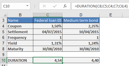
Comparison of Two Federal Securities (August 30, 2010)

Security	Nominal Interest	Maturity	Price	Yield	Duration
Federal Loan of 2005	3.25%	July 4, 2015	109.040	1.31%	4.54 years
Federal Medium-Term Bond Series 157	2.25%	April 10, 2015	104.500	1.24%	4.40 years

A calculation of the duration returns the following result:

Security	Duration
Federal loan of 2005	4.54 years
Federal medium-term bond series 157	4.40 years

The federal medium-term bond is preferable. However, the difference regarding the duration is very small. There is also another risk advantage for other debtors, and other terms as well as in regard to tax-related aspects (nominal interest must be reduced depending on the rate of taxation).

Interpretation:

• The medium-term bond (4.40 years) is preferable due to its shorter duration (lower risk).
• Limitations: Market conditions, credit risk, and tax implications may also influence decisions.

Converts a decimal number into a fractional representation where the decimal portion is expressed as a numerator over a specified denominator.

Syntax

DOLLARFR(Number; Factor)

Arguments

• Number (required)
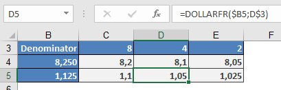
  The decimal number to convert (e.g., 8.25 → 8¼).
• Factor (required)
  The denominator of the fraction (must be a positive integer).
  • Truncates decimals (e.g., Factor = 4.9 → 4).
  • Errors:
    • #DIV/0! if Factor = 0.
    • #NUMBER! if Factor < 0.

Background

Historically, U.S. stock markets priced securities in fractions (e.g., ¼, ½, ⅛). This function reverts decimals to fractional notation for compatibility with legacy systems.

Example

Notes

• Formatting: The result displays as a decimal but represents a fraction (e.g., 8.1 = 8 + 1/4).
• Inverse Function: Use DOLLARDE() to convert fractional notation back to decimals.
• Precision: Truncates excess decimals (e.g., 1.13 with Factor = 8 → 1.1 = 1⅛).

Converts a fractional number (expressed with a decimal numerator) into a decimal value by applying a specified denominator.

Syntax

DOLLARDE(Number; Factor)

Arguments

• Number (required)
  The value whose decimal portion is treated as the numerator of a fraction.
  • Example: 1.1 with Factor = 2 → 1 + 1/2 = 1.5.
• Factor (required)
  The denominator of the fraction. Must be a positive integer (decimal places are truncated).
  • If Factor ≤ 0, returns:
    • #NUMBER! (for negative values).
    • #DIV/0! (if zero).

Background

Historically, U.S. stock markets used fractional pricing (e.g., 1¼ dollars). This function standardizes such values into decimals for easier comparison.

• Common denominators: 2 (halves), 4 (quarters), 8 (eighths), 16 (sixteenths).

Example

Input (Number)	Factor	Interpretation	Result (DOLLARDE)
1.1	2	1 + 1/2 = 1.5	1.5
1.1	4	1 + 1/4 = 1.25	1.25
1.1	8	1 + 1/8 ≈ 1.125	1.125
2.2	4	2 + 2/4 = 2.5	2.5
2.2	8	2 + 2/8 = 2.25	2.25

Notes

• Limitation: Decimals beyond the factor’s precision are ignored.
  • Example: 1.12 with Factor = 8 → Only 1.1 is read as 1 + 1/8 (=1.125).
• Inverse Function: Use DOLLARFR() to convert decimals back to fractional notation.

This function calculates the discount rate (anticipative interest rate) for a security based on its cash value, redemption value, and time to maturity (simple interest yield).

Syntax

DISC(Settlement; Maturity; Price; Repayment; [Basis])

Arguments

• Settlement (required)
  The date when the security is purchased.
  • Must be a valid date; time values are truncated.
• Maturity (required)
  The date when the security matures (redemption date).
  • Must be a valid date; time values are truncated.
• Price (required)
  The purchase price per $100 face value of the security.
  • Must be a positive number.
• Repayment (required)
  The redemption value per $100 face value at maturity.
  • Must be a positive number.
• Basis (optional)
  The day-count convention used for interest calculation.
  • If omitted, defaults to 0 (US (NASD) 30/360).

Error Handling

• If invalid dates or non-numeric values are provided, #VALUE! is returned.
• If invalid numbers (e.g., negative prices) are entered, #NUMBER! is returned.

Background

The anticipative interest method calculates yield upfront (discounting from the future value), unlike traditional interest calculations (yield in arrears).

• Common in short-term securities (e.g., treasury bills, commercial paper).
• The formula for the discount rate is derived from:

Discount Rate=Repayment−PriceRepayment×Days in YearDays to MaturityDiscount Rate=RepaymentRepayment−Price​×Days to MaturityDays in Year​

• Relationship to RECEIVED():
  DISC() and RECEIVED() are inverse functions, allowing conversion between anticipative and arrears interest rates.

Examples

1. Bill of Exchange Discounting
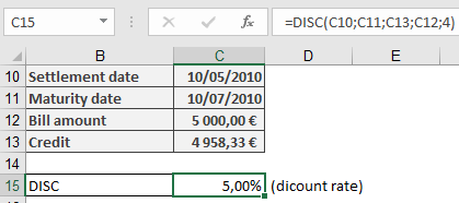
   • Scenario: A $5,000 bill of exchange with 2 months to maturity is discounted at $4,958.33.
   • Formula:

=DISC(« 10-May-2010 », « 10-Jul-2010 », 4958.33, 5000, 4)

1. • Result: 5% discount rate.

1. Treasury Bond Yield
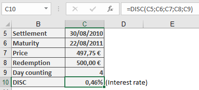
   • Scenario: A German treasury bond (face value €500) priced at €497.75 with 1-year maturity.
   • Formula:

=DISC(« 30-Aug-2010 », « 22-Aug-2011 », 497.75, 500, 4)

1. • Result: 0.46% annual discount rate.

Notes

• For tax or regulatory compliance, verify day-count conventions (Basis).
• Use YIELDDISC() or RECEIVED() for equivalent yield calculations.

This function calculates depreciation amounts using a multiple-rate (accelerated) depreciation method.

Syntax

DDB(Purchase_Value; Residual_Value; Life; Period; [Factor])

Arguments

• Purchase_Value (required)
  The purchase cost of an asset (net purchase price plus incidental expenses minus purchase cost reductions).
  • If a non-numeric value is provided, the #VALUE! error is returned.
  • If a negative number is entered, the #NUMBER! error is returned.
• Residual_Value (required)
  The value of the asset at the end of its depreciation period.
  • If a non-numeric value is provided, the #VALUE! error is returned.
  • If a negative number is entered, the #NUMBER! error is returned.
• Life (required)
  The number of periods over which the asset is depreciated.
  • Must be a positive integer.
• Period (required)
  The specific period within the depreciation duration for which the depreciation amount is calculated.
  • Must be a positive integer not exceeding the value of Life.
• Factor (optional)
  The multiplier applied to the straight-line depreciation rate (reciprocal of the depreciation duration).
  • If omitted, Excel uses a default value of 2 (double-declining balance method).

Background

Depreciation reflects the loss of an asset’s value over time and makes this loss visible. It should not be confused with wear-and-tear depreciation, which relates to the cost allocation of an asset as an operating expense from a tax perspective.

This method initially follows straight-line depreciation but applies an additional factor to the depreciation rate, making it a geometric (accelerated) depreciation.

• If the factor is 2, it is called the double-declining balance method.
• Higher factors result in faster depreciation in early periods.

Example

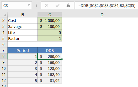
An asset with a purchase cost of $1,000.00 is depreciated over five years to a residual value of $100.00 using the double-declining balance method.

• The depreciation amount for each period can be calculated using DDB() and subtracted from the previous period’s book value.
• Alternatively, a custom depreciation schedule can be created, especially for tax-compliant methods, as built-in functions may not always apply.

This function calculates the depreciation amounts for an asset using the declining balance (geometric-degressive) depreciation method, accounting for partial years (in complete months) in the first depreciation period.

Syntax
DB(Purchase_Value; Residual_Value; Life; Period; [Months])

Arguments

• Purchase_Value (required)
  The purchase cost of an asset (net purchase price plus incidental expenses minus purchase cost reductions).
  • If a non-numeric value is provided, the #VALUE! error is returned.
  • If a negative number is entered, the #NUMBER! error is returned.
• Residual_Value (required)
  The value of the asset at the end of its depreciation period.
  • If a non-numeric value is provided, the #VALUE! error is returned.
  • If a negative number is entered, the #NUMBER! error is returned.
• Life (required)
  The number of periods over which the asset is depreciated.
  • Must be a positive integer.
• Period (required)
  The specific period within the depreciation duration for which the depreciation amount is calculated.
  • Must be a positive integer not exceeding the value of Life.
• Months (optional)
  Specifies the duration of a partial period in the purchase year (in complete months).
  • If omitted, Excel assumes a full year (12 months).

Background
Depreciation reflects the loss of an asset’s value over time and makes this loss visible. It should not be confused with wear-and-tear depreciation, which relates to the cost allocation of an asset as an operating expense from a tax perspective.

For the declining balance depreciation rate, the following formula applies:

Depreciation Rate=1−(Residual_ValuePurchase_Value)1LifeDepreciation Rate=1−(Purchase_ValueResidual_Value​)Life1​

This explains why a residual value of zero is impractical—depreciation would fully occur in the first year. In such cases, a residual value of $1,000.00 is typically assumed.

In Excel:

• Depreciation values are rounded to three decimal places.
• Each period’s depreciation is applied against the book value.
• The resulting depreciation amount reduces the book value for the next period.
• If the first period is shorter than a year, the depreciation rate is adjusted proportionally (divided by 12).

Example
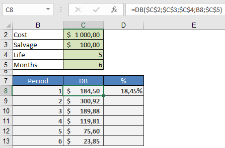
An asset with a purchase cost of $1,000.00 is depreciated over five years to a residual value of $100.00 using the declining balance method. The depreciation amount for each period can be calculated using DB() and subtracted from the previous period’s book value.

Alternatively, a depreciation schedule can be created by applying the formulas described above to compute the first depreciation amount and subsequent values.

This function calculates the principal portion repaid between two specified periods for an annuity loan (a loan repaid in equal periodic installments).

Syntax:

CUMPRINC(Rate, Nper; Pv; Start_Period; End_Period; Type)

Arguments:

• Rate (required): The nominal interest rate of the loan.
• Nper (required): The total number of repayment periods.
• Pv (required): The principal loan amount.
• Start_Period (required): The first period of the calculation.
• End_Period (required): The last period of the calculation.
• Type (required): The payment timing argument, where:
  • Type = 1 indicates payments are made at the beginning of each period.
  • Type = 0 (default) indicates payments are made at the end of each period.

Notes:

• If fractional values are provided for integer-based arguments (e.g., Start_Period), the decimals are truncated.
• Rate, Nper, and Pv must be positive; otherwise, CUMPRINC() returns the #NUM! error.
• Start_Period must be ≥ 1.
• End_Period must be ≥ 1 and ≥ Start_Period.
• Type must be 0 or 1.

Background:

Loans can be repaid in different ways. In an annuity repayment:

• The borrower pays a fixed amount each period, consisting of:
  • A principal repayment portion (increases over time).
  • An interest portion (decreases as the outstanding loan balance shrinks).

This function calculates the compounded principal repayment (excluding interest). By summing principal repayments over past periods, you can determine the residual debt (remaining loan balance).

Examples:

1. Principal Repayment Over a Loan Term
   In the Repayment Calculation (Annuity) example from the PV() function:
   • A borrower takes a $176,121.76 loan at 5.5% annual interest, repaying $1,000/month for 30 years.
   • By the 19th month, the residual debt is $172,513.25, meaning $3,608.51 of principal has been repaid.

Verify this with CUMPRINC() (accounting for rounding errors):

=-CUMPRINC(5.5%/12; 30*12; 176121.76; 1; 18; 0)

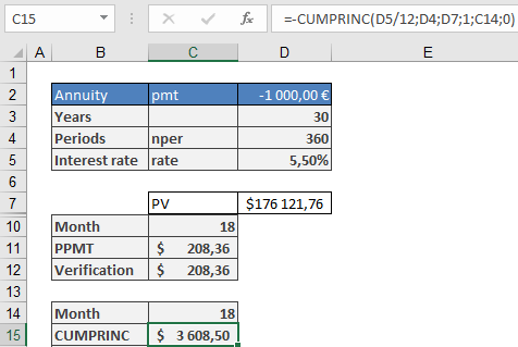
(Negative result indicates cash outflow relative to the loan amount.)

1. Fixed-Rate Mortgages & Residual Debt
   Many mortgage loans have a fixed interest rate for an initial period (shorter than the full term).
   • Borrowers can use CUMPRINC() to calculate residual debt after the fixed-rate period.
   • This helps assess refinancing risks if interest rates rise.
   • Example calculation method matches the previous example.

Rounding Considerations:

Built-in functions may not reflect real-world bank calculations (which use 2 decimal places). For precise repayment schedules, use the ROUND() function in monthly plans.

This function calculates the accrued interest paid between two specified periods for an annuity loan (a loan repaid in equal periodic installments).

Syntax:
CUMIPMT(Rate, Nper; Pv; Start_Period; End_Period; Type)

Arguments:

• Rate (required): The nominal interest rate of the loan.
• Nper (required): The total number of repayment periods.
• Pv (required): The principal loan amount.
• Start_Period (required): The first period of the calculation.
• End_Period (required): The last period of the calculation.
• Type (required): The payment timing argument, where:
  • Type = 1 indicates payments are made at the beginning of each period.
  • Type = 0 (default) indicates payments are made at the end of each period.

Notes:

• If fractional values are provided for integer-based arguments (e.g., Start_Period), the decimals are truncated.
• Rate, Nper, and Pv must be positive; otherwise, CUMIPMT() returns the #NUM! error.
• Start_Period must be ≥ 1.
• End_Period must be ≥ 1 and ≥ Start_Period.
• Type must be 0 or 1.

Background:
Loans can be repaid in different ways. In an annuity repayment, the borrower pays a fixed amount each period, consisting of:

• A repayment portion (increases over time).
• An interest portion (decreases as the outstanding loan balance shrinks).

While summing partial repayments is valid (to determine residual debt), summing interest payments lacks financial-mathematical significance. It is commonly used for loan comparisons (even by financial institutions), but it does not reflect a true financial analysis. Interest totals are meaningful only when evaluated at the loan’s origination. For example, a $100,000 loan requires repayment of the principal plus accrued interest if repaid later.

Example:
In the Repayment Calculation (Annuity) example from the PV() function:

• A borrower takes a $176,121.76 loan at 5.5% annual interest, repaying $1,000/month for 30 years.
• By the 19th month, the residual debt is $172,513.25, indicating $3,608.51 has been repaid. Thus, the interest paid is:
  $18,000 (total paid) – $3,608.51 (principal) = $14,391.49 (interest).

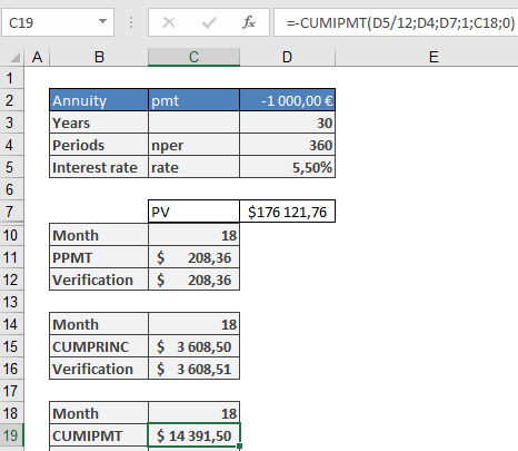
This can be verified with CUMIPMT() (accounting for rounding errors):

=-CUMIPMT(5.5%/12, 30*12, 176121.76, 1, 18, 0)

(Negative result indicates cash outflow relative to the loan amount.)

Rounding Considerations:
Built-in functions may not reflect real-world bank calculations (which use 2 decimal places). For precise repayment schedules, use the ROUND() function in monthly plans.

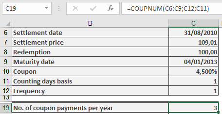
This function calculates the number of coupon payments (interest payment dates) remaining after the settlement date—i.e., how many interest payments the new owner of a fixed-interest security will receive until maturity.

Syntax. COUPNUM(Settlement; Maturity; Frequency; Basis)
Arguments

• Settlement (required): The date on which the bond is purchased or transferred (ownership changes).
• Maturity (required): The date on which the bond will be repaid (the loan ends).
• Frequency (required): Specifies the number of coupon payments per year. Valid values:
  • 1 = Annual payments
  • 2 = Semiannual (every six months)
  • 4 = Quarterly (every three months)
• Basis (optional): Defines the day count basis used for calculations. If omitted, Excel uses Basis = 0.
  Refer to Table 15-2 for available basis options:
  • 0 = US (NASD) 30/360
  • 1 = Actual/actual
  • 2 = Actual/360
  • 3 = Actual/365
  • 4 = European 30/360

Argument Requirements & Errors

• Date values must not include time components; any decimal portion is truncated.
• The Frequency and Basis values are also truncated to integers.
• If Settlement or Maturity is not a valid date, the function returns a #VALUE! error.
• If Frequency is not 1, 2, or 4, or if Basis is not in the range 0–4, the function returns a #NUM! error.
• If the Settlement date is later than the Maturity date, the function also returns a #NUM! error.

Background

For fixed-interest securities (bonds), coupon payments are made regularly according to the maturity date and payment frequency.
The COUPNUM() function determines how many of these payments are left after the bond is purchased.

This result is useful when calculating the present value of future payments, such as when determining the bond’s PRICE() or YIELD() at purchase.
Note that the day count basis (Basis argument) can affect results, especially for partial-year (intra-annual) periods.

Example

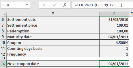
Returns the next coupon payment date after the settlement date for a fixed-income security with regular interest payments.

Syntax

COUPNCD(Settlement; Maturity; Frequency; Basis)

Arguments

Argument	Required	Description	Valid Values
Settlement	Yes	Date of ownership transfer	Valid Excel date
Maturity	Yes	Bond repayment date	Must be after Settlement
Frequency	Yes	Interest payments per year	1 (annual), 2 (semi-annual), 4 (quarterly)
Basis	No	Day-count convention	0-4 (default=0)

Day-Count Basis Methods (Table 1)

Basis	Method	Common Usage
0	30/360 (NASD)	Corporate bonds
1	Actual/Actual	Government securities
2	Actual/360	Money market instruments
3	Actual/365	UK gilts
4	30/360 (European)	Eurobonds

Requirements & Error Handling

• Dates must be valid (time components are ignored)
• Frequency and Basis are converted to integers
• Returns #VALUE! for invalid date formats
• Returns #NUM! for:
  • Invalid Frequency (not 1, 2, or 4)
  • Invalid Basis (not 0-4)
  • Settlement date ≥ Maturity date

Background

• Critical for determining future cash flows
• Used in conjunction with:
  • COUPDAYSNC() (days to next coupon)
  • COUPPCD() (previous coupon date)
• Different day-count methods may yield different coupon date calculations

Example Applications

Key Notes

• For US corporate bonds: Typically Basis=0
• For Treasury securities: Typically Basis=1
• Always verify Settlement precedes Maturity
• Combine with COUPNUM() for complete coupon analysis
• Critical for bond portfolio management between payment dates

Common Errors

1. Using text strings instead of date serials
2. Incorrect Frequency for bond type
3. Mismatching Basis with market convention

Note: Refer to RATE() and YIELD() function examples for implementation scenarios.