Votre panier est actuellement vide !
Catégorie : Excel function
How to use the VARA() function in Excel
This function estimates the variance based on a sample. Unlike VAR.S(), VARA() includes numbers, text, and logical values (TRUE/FALSE) in the calculation.
Syntax. VARA(value1; value2; …)
Arguments- value1 (required) and
- value2 (optional)
You can enter at least one and up to 255 values (limited to 30 in Excel 2003 and earlier), which make up a sample from the population.
Background
The only distinction between VARA() and VAR.S() is that VARA() includes text and logical values in its computation. For this reason, the focus here is on VARA().
VARA() uses the same formula as VAR.S():
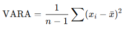
Where:
- xˉ is the sample mean, calculated as AVERAGE(value1; value2; …)
- n is the total number of values in the sample
In VARA(), text entries and the logical value FALSE are treated as 0, and TRUE is treated as 1.
Example
Let’s revisit the evaluation of website visits. Over the past 18 months, the company experienced technical issues that affected visit tracking. Specifically:
- In May 2007 and August 2007, hosting problems caused the website to be unavailable. These months are marked with the text « hostingproblems ».
- In March 2008, changes to the product section restricted access. This is represented by the logical value FALSE.
As shown in Figure below, the VARA() function returns a different result from VAR.S()—this is because VARA() incorporates both text and logical values in its variance calculation.
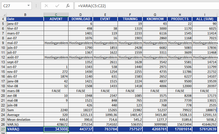
In this case:
- The text values (« hostingproblems ») and the logical value FALSE are both counted as 0 in the calculation.
By examining the DOWNLOAD section, the result can be summarized as follows:
The average squared deviation from the mean—including text and logical values—is 443,737 for the DOWNLOAD area.
How to use the VAR.S() function in Excel
This function estimates the variance based on a sample of the population. VAR.S() measures how the data points are distributed around the mean.
Syntax. VAR.S(number1; number2; …)
Arguments- number1 (required) and
- number2 (optional)
You can enter at least one and up to 255 numeric arguments, which represent a sample of the population.
Background
In statistics, the two most commonly used measures of data spread are variance and standard deviation.
- Variance quantifies the average squared deviation of a variable x from its expected value E(x).
- This result is known as the empirical variance.
There are two types of variance:
- Population variance: Measures the spread within an entire population. Use the function VAR.P() for this.
- Sample variance: Measures the spread within a sample from a population. This is commonly used in descriptive statistics to describe data spread and in inferential statistics to estimate population variance. Use the function VAR.S() for this.
When working with a sample, the sum of the squared deviations is divided by (n – 1) instead of n to correct for bias.
VAR.S() uses the following formula: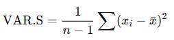
Where:
- xˉ is the sample mean, calculated by AVERAGE(number1; number2; …)
- n is the number of data points in the sample
Note: Squaring the deviations gives more weight to extreme values, which may influence the result.
A key limitation of variance is that it uses squared units, which differ from the original data units. For this reason, the standard deviation, which is the square root of the variance, is often used for interpretation.
Example
Because sample variance reflects how widely data points are spread, it is widely used in descriptive statistics.
In this example, the marketing department of a software company uses the VAR.S() function to analyze website visit data. The objective is to gain clearer insights and improve performance across different sections of the site.
Important: The analyzed data represents a sample — although the website has been online for a long time, the analysis only includes data from 18 months (January 2007 to June 2008).
As shown in Figure below, the department calculates the variance, the mean, and the average deviation.
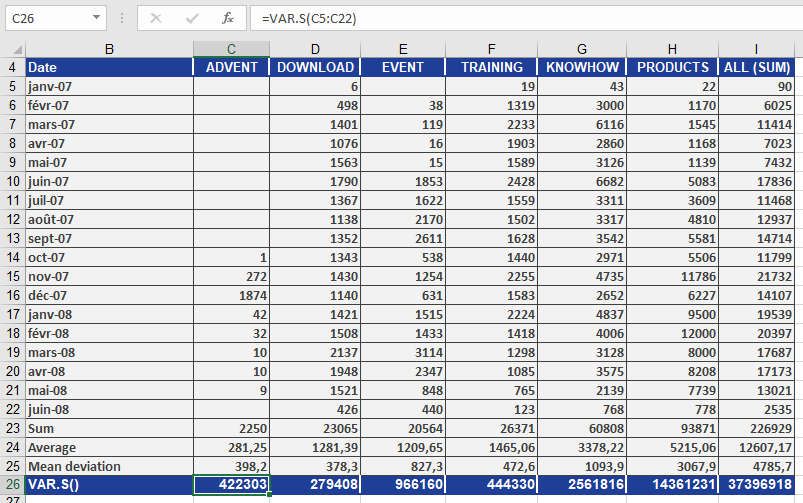
By examining the DOWNLOAD section, you can make the following statement:
The average squared deviation from the arithmetic mean for the DOWNLOAD area is 279,408.
How to use the VAR.P() function in Excel
This function calculates the variance assuming that the entire data set represents the whole population.
Syntax. VAR.P(number1; number2; …)
Arguments- number1 (required) and
- number2 (optional)
You can enter at least one and up to 255 numeric arguments, which represent the population data set.
Background
The only difference between VAR.P() and VAR.S() lies in how they treat the data set:
- VAR.P() calculates the population variance,
- while VAR.S() is based on a sample from the population.
This example focuses on VAR.P(). For more details about variance and the sample-based function, refer to the VAR.S() description.
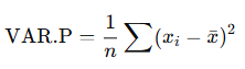
The formula used by VAR.P() is:
Where:
- xˉ is the population mean, calculated using AVERAGE(number1, number2, …)
- n is the total number of data points in the population
Example
Let’s return to the website analysis of the software company (see Figure below).
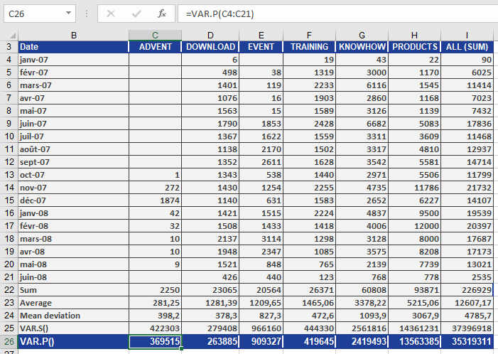
Since VAR.P() and VAR.S() use different formulas, they produce different results (as shown in Figure above).
Looking specifically at the DOWNLOAD data section, you can conclude the following:The average squared deviation from the arithmetic mean (based on the entire population) is 263,885.
How to use the TRIMMEAN() function in Excel
This function returns the average value of a data group, excluding the values from the top and bottom of the data set.
TRIMMEAN() calculates the average of a subset of data points, excluding the smallest and largest values of the original data points based on the specified percentage. Use this function to exclude outlying data from your analysis.
Syntax
TRIMMEAN(array; percent)
Arguments
- array (required) – The array or range of values to trim and average.
- percent (required) – The percentage of data points to exclude from the calculation. For example, if percent = 0.2, four points are trimmed from a data set of 20 points (20 × 0.2): two from the top and two from the bottom of the set.
Background
Usually, all values in a data set are used to calculate the mean. However, you might want to exclude the marginal areas to calculate a mean without outliers, resulting in a trimmed mean.
If the data contains outliers—that is, a few values that are too high or too low—sort the observed values in ascending order, trim the values at the beginning and end, and calculate the mean from the remaining values.
To get a mean trimmed by 10 percent, omit 5 percent of the values at the beginning and 5 percent at the end.
Example
You are the executive manager of the controlling department of a software company and have compiled the sales for the past 17 months, from January 2007 to May 2008. You want to calculate the average sales and exclude outliers, so you sort the sales in ascending order.
- If you use the AVERAGE() function, the result is not meaningful because the outliers are included in the calculation and skew the result.
- The MEDIAN() function also doesn’t return the correct result.
- Therefore, you use the TRIMMEAN() function.
As shown in Figure below, the calculation of the average sales returns a higher value due to the outliers.
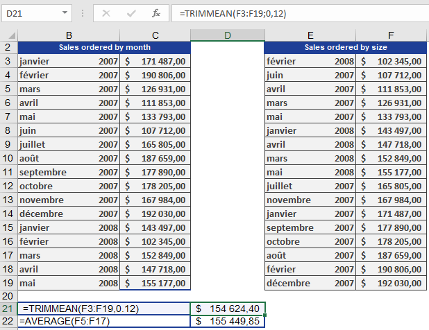
You specify 0.12 for the percent argument. This means that 12% of the original values are excluded from the calculation (6% from the top and 6% from the bottom). The trimmed mean returns an average sale of $154,624.40.
How to use the TREND() function in Excel
This function returns values along a linear trend. TREND() fits a straight line (using the least squares method) to the arrays of known_y’s and known_x’s. It then returns the corresponding y-values along that line for the specified array of new_x’s.
Syntax. TREND(known_y’s; known_x’s; new_x’s; const)
Argumentsknown_y’s (required): The known y-values in the equation y = mx + b:
— If the known_y’s array is a single column, each column in known_x’s is treated as a separate variable.
— If the known_y’s array is a single row, each row in known_x’s is interpreted as a separate variable.known_x’s (optional): The known x-values in the equation y = mx + b:
— This array may contain one or more sets of variables. If there’s only one variable, known_y’s and known_x’s can be ranges of any shape as long as they have matching dimensions. If there is more than one variable, known_y’s must be a vector (a single row or column).
— If known_x’s is omitted, it defaults to the array {1, 2, 3, …} with the same number of elements as known_y’s.
— known_y’s and known_x’s must have the same number of rows or columns. A mismatch leads to a #REF! error. A zero or negative y-value will produce a #NUM! error.new_x’s (optional): The new x-values for which you want the function to return the corresponding y-values:
— Like known_x’s, new_x’s must have one column (or row) for each independent variable. If known_y’s is a single column, then known_x’s and new_x’s must have the same number of columns. If known_y’s is a single row, then known_x’s and new_x’s must have the same number of rows.
— If new_x’s is not provided, it is assumed to be equal to known_x’s.
— If both known_x’s and new_x’s are omitted, Excel assumes them to be {1, 2, 3, …} with the same number of elements as known_y’s.const (optional): A logical value that specifies whether to force the constant b to equal 1:
— If const is TRUE or omitted, b is calculated normally.
— If const is FALSE, b is set to 1, and the slope m is adjusted so the formula becomes y = m^x.Background
When you know that some values are interdependent, you can use TREND() to make predictions based on known data.
Excel provides several statistical functions for calculating trends. These functions determine a line or curve from existing values. By extending the timeline, you can forecast future values. Known values are analyzed and expressed as a formula for extrapolation. However, your dataset must be large enough to account for seasonal patterns. Unpredictable influences can also distort trend predictions.Example: Suppose a competitor launches a highly successful new product in your area. This sudden change could disrupt your data model. Since regression analysis approximates data using mathematical functions, Excel includes various tools for this, including the TREND() function.
Use TREND() to identify a linear trend or analyze existing data. The values are plugged into a formula to help you forecast future changes.
The x- and y-values come from the equation y = mx + b, where:
— b is the y-intercept (where the line crosses the y-axis), and
— m is the slope (the rate of change of y for every unit change in x).
If changes follow a consistent pattern, a linear trend exists.Example
You’re the marketing manager of a software company analyzing web traffic. Recently, both visits and online orders have significantly increased. You want to forecast future activity, so you use the TREND() function to project future values.
The website visits and orders up to June 2008 are shown in Figure below.

You generate a chart from the available data to visualize the linear trend for website visits and online orders. The chart includes equations and the coefficient of determination (r²), as shown in Figure below.
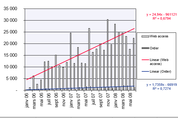
The linear trend line and equation show that orders increase by 52.872 each month — roughly 53 new orders per month.
You now want to project the trend for visits and orders from July 2008 to March 2009.To calculate website visits over the next nine months, use these TREND() arguments:
- known_y’s = website visits from January 2008 to June 2008
- known_x’s = months from January 2006 to June 2008
- new_x’s = months from July 2008 to March 2009
- const = TRUE (calculate b normally in the equation y = mx + b)
Figure below displays the results.

By applying the same method, you can forecast online orders using the projected website visits. Figure below shows the calculated values and the arguments used in the TREND() function.
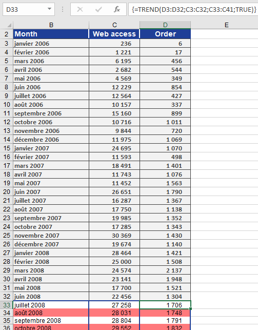
With the TREND() function, Excel allows accurate forecasting of website visits and online orders, assuming the previous exponential growth trend continues.
How to use the T.TEST() function in Excel
The T.TEST() function returns the probability (p-value) associated with a Student’s t-test. It evaluates whether the means of two data sets are statistically different from each other. Use this function to determine if the two samples likely come from populations with the same mean.
Syntax
T.TEST(array1; array2; tails; type)
Arguments
- array1 (required):
First sample data set. - array2 (required):
Second sample data set. - tails (required):
Specifies the number of distribution tails:- 1 = One-tailed test
- 2 = Two-tailed test
- type (required):
Type of t-test to perform:- 1: Paired sample t-test
- 2: Two-sample equal variance (homoscedastic)
- 3: Two-sample unequal variance (heteroscedastic)
Background
The Student’s t-distribution is used when sample sizes are small and the population standard deviation is unknown. It is symmetrical and bell-shaped but has heavier tails than the normal distribution. It is parameterized by degrees of freedom.
The t-test determines the likelihood that the difference between sample means occurred by chance.
The general t-test formula is:
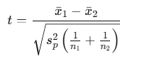
Where:
- xˉ1,xˉ2 are the sample means
- sp2s_p^2sp2 is the pooled variance (used if variances are equal)
- n1,n2 are sample sizes
Types of t-tests
- Paired Sample t-test (type = 1)
Used when the same subjects are measured twice (e.g., before and after treatment).
- Two-sample Equal Variance t-test (type = 2)
Used when two independent samples are assumed to have equal variances.
- Two-sample Unequal Variance t-test (type = 3)
Used when two independent samples have unequal variances.
Tails
- One-tailed test (tails = 1):
Tests if the mean of one sample is greater than or less than the other. - Two-tailed test (tails = 2):
Tests if the means are significantly different in either direction.
Hypotheses
One-tailed test:
- H0:μ1≤μ2
- H1:μ1>μ2
Two-tailed test:
- H0:μ1=μ2
- H1:μ1≠μ2
Example
A drug company runs a clinical study to test if a higher dosage of a treatment accelerates recovery. Two groups are observed:
- Group 1 receives the standard dosage
- Group 2 receives the increased dosage
You want to test the hypothesis that Group 2 recovers faster than Group 1.
You perform a one-tailed, two-sample equal variance t-test with:
T.TEST(array1, array2, 1, 2)
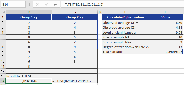
Assume the result is 0.014 (1.4%).
Interpretation
- The p-value = 0.014, which is less than the significance level α = 0.05.
- ⇒ Reject the null hypothesis.
- ⇒ There’s strong evidence that Group 2 recovers faster than Group 1.
Key Points
- If T.TEST() result < α (e.g., 0.05), the difference is statistically significant.
- The function outputs a probability, not a t-value.
- T.TEST() is more accurate and preferred over manual lookup of critical t-values.
Note: T.TEST() replaces the older TTEST() function in newer Excel versions, but both work the same.
- array1 (required):
How to use the T.INV.2T() function in Excel
This function returns the t-value of the t-distribution based on a given probability and degrees of freedom.
Syntax:
T.INV.2T(probability; degrees_freedom)Arguments:
- probability (required) – The probability associated with the two-tailed Student’s t-distribution.
- degrees_freedom (required) – The number of degrees of freedom characterizing the distribution.
NOTE:
- If any argument is non-numeric, T.INV.2T() returns the #VALUE! error.
- If probability is < 0 or > 1, T.INV.2T() returns the #NUM! error.
- If degrees_freedom is not an integer, it is truncated. If degrees_freedom is < 1, the function returns #NUM!.
- T.INV.2T() returns the value t, such that P(|X| > t) = probability, where X is a random variable following the t-distribution, and P(|X| > t) = P(X < –t or X > t).
Key Points:
- A quantile of the t-distribution can be interpreted as the t-value of a one-tailed confidence interval. Due to the symmetry of the t-distribution, the t-value for a one-tailed interval can be calculated by replacing probability with 2*probability.
- For a probability of 0.05 and 10 degrees of freedom, the two-tailed t-value is calculated as:
=T.INV.2T(0.05, 10) → 2.28139. - The one-tailed t-value for the same parameters is:
=T.INV.2T(2*0.05, 10) → 1.812462. - If probability is specified, T.INV.2T() finds x such that T.DIST.2T(x, degrees_freedom, 2) = probability. Thus, its accuracy depends on T.DIST.2T().
- The function uses an iterative search technique. If convergence fails after 100 iterations, it returns #N/A.
Background:
The t-value (critical value) returned by T.INV.2T() is used as a test statistic for hypothesis testing. It helps evaluate the null hypothesis.- Arguments:
- probability = significance level (calculable via T.DIST.2T()). For a one-tailed t-test, this level is doubled.
- degrees_freedom = (sum of both sample sizes) – 2.
Example:
A clinical study examines a drug’s efficacy:- Group 1: Normal dosage.
- Group 2: Increased dosage (one participant dropped out).
- Goal: Determine if the higher dosage speeds up recovery (measured in days).
Hypotheses:
- Null (H₀): No difference in treatment success between groups.
- Alternative (H₁): Group 2 recovers faster due to more effective treatment.
Test Setup:
- One-tailed t-test (type 2) comparing two independent sample means.
- Significance level (α): 0.05.
- Critical value calculation: =T.INV.2T(2*0.05; degrees_freedom).
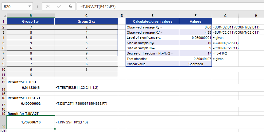
Result:
The critical t-value for the sample is 1.7396, which serves as a statistic to assess the null hypothesis.How to use the T.DIST.RT() function in Excel
This function returns the right-tailed Student’s t-distribution. The t-distribution is used for hypothesis testing with small sample data sets. Use this function instead of referring to a table of critical values for the t-distribution.
Syntax:
T.DIST.RT(x; degrees_freedom)Arguments:
- x(required): The numeric value at which to evaluate the distribution.
- degrees_freedom(required): An integer indicating the number of degrees of freedom.
Background:
For more details on t-distributed random variables, refer to the documentation for T.TEST().Example:
For further examples and usage of this function, see the figure below.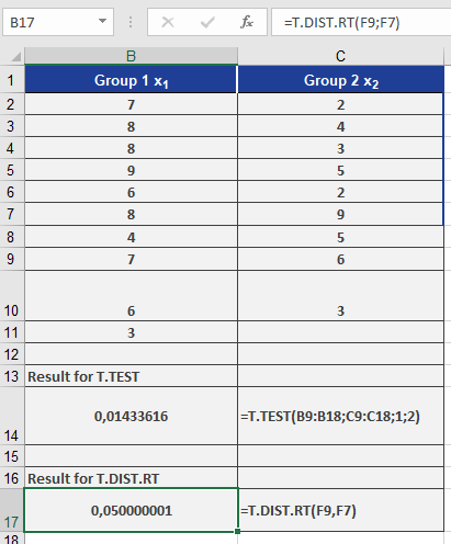
How to use the T.DIST.2T() function in Excel
This function returns the two-tailed distribution (1 – α) of a Student’s t-distributed random variable. The t-distribution is used for hypothesis testing with small sample data sets. Use this function instead of a table of critical values for the t-distribution.
Syntax:
T.DIST.2T(x; degrees_freedom)Arguments:
- x(required): The distribution value (quantile) for which you want to calculate the probability.
- degrees_freedom(required): An integer indicating the number of degrees of freedom.
Background:
The T.DIST.2T() function calculates the significance level (α-risk) of a t-distributed random variable. The probability of a hypothesis is evaluated based on this significance level.The significance level calculation becomes particularly useful when you:
- Calculate the critical value for a sample, then
- Use DIST.2T()to determine the significance level for that critical value.
The result from T.DIST.2T() helps determine whether the null hypothesis holds.
Example:
A clinical study examines drug efficacy:- Group 1:Standard daily dosage
- Group 2:Increased initial dosage
(One participant withdrew early for personal reasons)
Objective: Determine if the higher dosage accelerates recovery (measured in treatment days).
- Null Hypothesis (H₀):No difference in treatment effectiveness between groups.
- Alternative Hypothesis (H₁):Group 2 recovers faster due to more effective treatment.
A two-tailed, type 2 t-test (comparing means of independent samples) is conducted. T.DIST.2T() calculates the significance level for the critical value to evaluate the hypotheses.
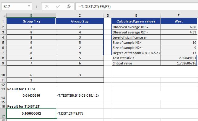
Result Interpretation:
If T.DIST.2T() returns 10% (0.1), this indicates:- There’s a 10% probability that the null hypothesis is valid.
- Since this probability is small (typically <5% is considered significant), we reject the null hypothesis.
How to use the STEYX() function in Excel
The STEYX() function calculates the standard error of the predicted y-values for each corresponding x-value in a linear regression.
This standard error quantifies the accuracy of the predictions — the smaller the standard error, the more reliable the regression model.
Syntax:
STEYX(known_y’s; known_x’s)
Arguments
- known_y’s (required): A range or array of dependent data points (output or response values)
- known_x’s (required): A range or array of independent data points (input or predictor values)
Important:
The order matters — known_y’s must come first.Background
In statistics, the standard error represents the variation of a sample estimate (like a regression prediction) around the true population parameter. It is defined as the standard deviation of the sampling distribution.
- A small standard error implies that the predicted values are close to the true values
- A large standard error means there’s more uncertainty in the predictions
The standard error decreases as the sample size increases, approximately following this rule:
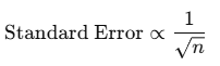
Where:
- n is the sample size
Thus, to halve the standard error, you’d need to quadruple the sample size.
Formula
The standard error of the predicted y-values is calculated using this general formula:
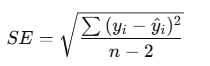
Where:
- yi = actual dependent value
- y^i = predicted y-value from the regression line
- n = number of data points
- The denominator n−2n – 2n−2 reflects the degrees of freedom in simple linear regression
Example
You’re a marketing manager at a software company. Your team records:
- Website visits (x-values) — independent variable
- Online orders (y-values) — dependent variable
Although the company is 10 years old, data from the last 2.5 years is available. You want to assess the reliability of using website visits to predict online orders.
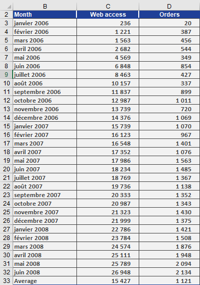
You’ve entered both series into Excel as seen below.
To find the standard error of the regression, use:
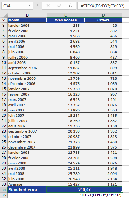
STEYX(Orders, Visits)
In your case:
- Mean of online orders yˉ=1,121\bar{y} = 1,121yˉ=1,121 (between July 2007 and June 2008)
- The function returns:
Result: 210.07
Interpretation
The value 210.07 means:
- On average, the predicted number of online orders deviates from the actual orders by about 210 orders.
- This indicates the expected margin of error in your predictions using the linear model.
Conclusion
Use the STEYX() function when:
- You’re performing linear regression
- You need to evaluate prediction accuracy
- You’re calculating confidence intervals or forecasting based on a known relationship between variables
The smaller the result, the tighter and more reliable your regression predictions will be.